3 Multiple regression

The general model for single-level data with $m$ predictors is

\[ Y_i = \beta_0 + \beta_1 X_{1i} + \beta_2 X_{2i} + \ldots + \beta_m X_{mi} + e_i \]

with $e_i \sim \mathcal{N}\left(0, \sigma^2\right)$—in other words, with the assumption that the errors are from a normal distribution having a mean of zero and variance $\sigma^2$.

Note that the key assumption here is not that the response variable (the $Y$s) is normally distributed, nor that the individual predictor variables (the $X$s) are normally distributed; it is only that the model residuals are normally distributed (for discussion, see this blog post). The individual $X$ predictor variables can be any combination of continuous and/or categorical predictors, including interactions among variables. Further assumptions behind this particular model are that the relationship is "planar" (can be described by a flat surface, analogous to the linearity assumption in simple regression) and that the error variance is independent of the predictor values.

The $\beta$ values are referred to as regression coefficients. Each $\beta_h$ is interpreted as the partial effect of $\beta_h$ holding constant all other predictor variables. If you have $m$ predictor variables, you have $m+1$ regression coefficients: one for the intercept, and one for each predictor.

Although discussions of multiple regression are common in statistical textbooks, you will rarely be able to apply the exact model above. This is because the above model assumes single-level data, whereas most psychological data is multi-level. However, the fundamentals are the same for both types of datasets, so it is worthwhile learning them for the simpler case first.

3.1 An example: How to get a good grade in statistics

Let's look at some (made up, but realistic) data to see how we can use multiple regression to answer various study questions. In this hypothetical study, you have a dataset for 100 statistics students, which includes their final course grade (grade), the number of lectures each student attended (lecture, an integer ranging from 0-10), how many times each student clicked to download online materials (nclicks) and each student's grade point average prior to taking the course, GPA, which ranges from 0 (fail) to 4 (highest possible grade).

3.1.1 Data import and visualization

Let's load in the data grades.csv and have a look.

library("corrr") # correlation matrices
library("tidyverse")

grades <- read_csv("data/grades.csv", col_types = "ddii")

grades

## # A tibble: 100 × 4
##    grade   GPA lecture nclicks
##    <dbl> <dbl>   <int>   <int>
##  1  2.40 1.13        6      88
##  2  3.67 0.971       6      96
##  3  2.85 3.34        6     123
##  4  1.36 2.76        9      99
##  5  2.31 1.02        4      66
##  6  2.58 0.841       8      99
##  7  2.69 4           5      86
##  8  3.05 2.29        7     118
##  9  3.21 3.39        9      98
## 10  2.24 3.27       10     115
## # ℹ 90 more rows

First let's look at all the pairwise correlations.

grades %>%
  correlate() %>%
  shave() %>%
  fashion()

## Correlation computed with
## • Method: 'pearson'
## • Missing treated using: 'pairwise.complete.obs'

##      term grade  GPA lecture nclicks
## 1   grade                           
## 2     GPA   .25                     
## 3 lecture   .24  .44                
## 4 nclicks   .16  .30     .36

pairs(grades)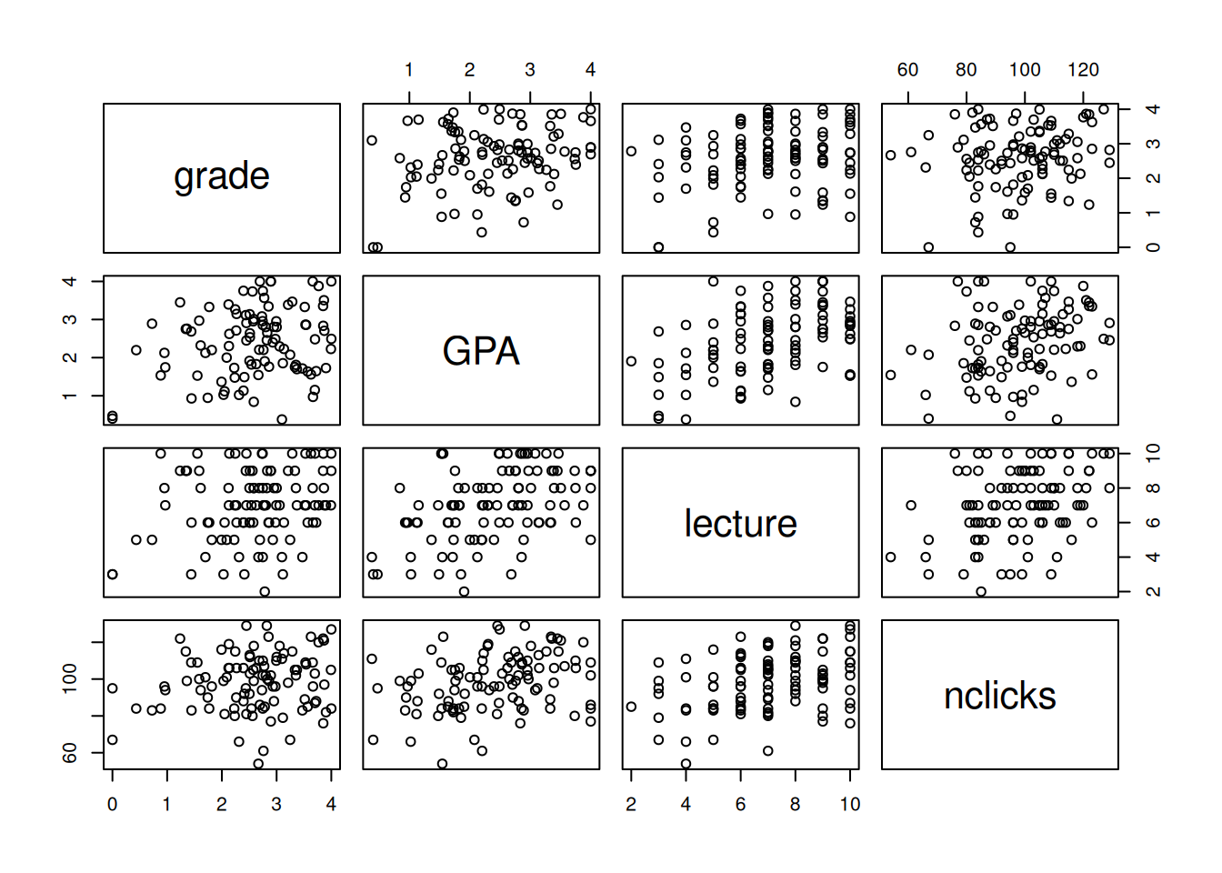

Figure 2.2: All pairwise relationships in the grades dataset.

3.1.2 Estimation and interpretation

To estimate the regression coefficients (the $\beta$s), we will use the lm() function. For a GLM with $m$ predictors:

\[ Y_i = \beta_0 + \beta_1 X_{1i} + \beta_2 X_{2i} + \ldots + \beta_m X_{mi} + e_i \]

The call to base R's lm() is

lm(Y ~ X1 + X2 + ... + Xm, data)

The Y variable is your response variable, and the X variables are the predictor variables. Note that you don't need to explicitly specify the intercept or residual terms; those are included by default.

For the current data, let's predict grade from lecture and nclicks.

my_model <- lm(grade ~ lecture + nclicks, grades)

summary(my_model)

## 
## Call:
## lm(formula = grade ~ lecture + nclicks, data = grades)
## 
## Residuals:
##      Min       1Q   Median       3Q      Max 
## -2.21653 -0.40603  0.02267  0.60720  1.38558 
## 
## Coefficients:
##             Estimate Std. Error t value Pr(>|t|)  
## (Intercept) 1.462037   0.571124   2.560   0.0120 *
## lecture     0.091501   0.045766   1.999   0.0484 *
## nclicks     0.005052   0.006051   0.835   0.4058  
## ---
## Signif. codes:  0 '***' 0.001 '**' 0.01 '*' 0.05 '.' 0.1 ' ' 1
## 
## Residual standard error: 0.8692 on 97 degrees of freedom
## Multiple R-squared:  0.06543,    Adjusted R-squared:  0.04616 
## F-statistic: 3.395 on 2 and 97 DF,  p-value: 0.03756

We'll often write the parameter symbol with a little hat on top to make clear that we are dealing with estimates from the sample rather than the (unknown) true population values. From above:

$\hat{\beta}_0$ = 1.46
$\hat{\beta}_1$ = 0.09
$\hat{\beta}_2$ = 0.01

This tells us that a person's predicted grade is related to their lecture attendance and download rate by the following formula:

grade = 1.46 + 0.09 $\times$ lecture + 0.01 $\times$ nclicks

Because $\hat{\beta}_1$ and $\hat{\beta}_2$ are both positive, we know that higher values of lecture and nclicks are associated with higher grades.

So if you were asked, what grade would you predict for a student who attends 3 lectures and downloaded 70 times, you could easily figure that out by substituting the appropriate values.

grade = 1.46 + 0.09 $\times$ 3 + 0.01 $\times$ 70

which equals

grade = 1.46 + 0.27 + 0.7

and reduces to

grade = 2.43

3.1.3 Predictions from the linear model using `predict()`

If we want to predict response values for new predictor values, we can use the predict() function in base R.

predict() takes two main arguments. The first argument is a fitted model object (i.e., my_model from above) and the second is a data frame (or tibble) containing new values for the predictors.

You need to include all of the predictor variables in the new table. You’ll get an error message if your tibble is missing any predictors. You also need to make sure that the variable names in the new table exactly match the variable names in the model.

Let's create a tibble with new values and try it out.

## a 'tribble' is a way to make a tibble by rows,
## rather than by columns. This is sometimes useful
new_data <- tribble(~lecture, ~nclicks,
                    3, 70,
                    10, 130,
                    0, 20,
                    5, 100)

The tribble() function provides a way to build a tibble row by row, whereas with tibble() the table is built column by column.

The first row of the tribble() contains the column names, each preceded by a tilde (~).

This is sometimes easier to read than doing it row by row, although the result is the same. Consider that we could have made the above table using

new_data <- tibble(lecture = c(3, 10, 0, 5),
                   nclicks = c(70, 130, 20, 100))

Now that we've created our table new_data, we just pass it to predict() and it will return a vector with the predictions for $Y$ (grade).

predict(my_model, new_data)

##        1        2        3        4 
## 2.090214 3.033869 1.563087 2.424790

That's great, but maybe we want to line it up with the predictor values. We can do this by just adding it as a new column to new_data.

new_data %>%
  mutate(predicted_grade = predict(my_model, new_data))

## # A tibble: 4 × 3
##   lecture nclicks predicted_grade
##     <dbl>   <dbl>           <dbl>
## 1       3      70            2.09
## 2      10     130            3.03
## 3       0      20            1.56
## 4       5     100            2.42

Want to see more options for predict()? Check the help at ?predict.lm.

3.1.4 Visualizing partial effects

As noted above the parameter estimates for each regression coefficient tell us about the partial effect of that variable; it's effect holding all of the others constant. Is there a way to visualize this partial effect? Yes, you can do this using the predict() function, by making a table with varying values for the focal predictor, while filling in all of the other predictors with their mean values.

For example, let's visualize the partial effect of lecture on grade holding nclicks constant at its mean value.

nclicks_mean <- grades %>% pull(nclicks) %>% mean()

## new data for prediction
new_lecture <- tibble(lecture = 0:10,
                      nclicks = nclicks_mean)

## add the predicted value to new_lecture
new_lecture2 <- new_lecture %>%
  mutate(grade = predict(my_model, new_lecture))

new_lecture2

## # A tibble: 11 × 3
##    lecture nclicks grade
##      <int>   <dbl> <dbl>
##  1       0    98.3  1.96
##  2       1    98.3  2.05
##  3       2    98.3  2.14
##  4       3    98.3  2.23
##  5       4    98.3  2.32
##  6       5    98.3  2.42
##  7       6    98.3  2.51
##  8       7    98.3  2.60
##  9       8    98.3  2.69
## 10       9    98.3  2.78
## 11      10    98.3  2.87

Now let's plot.

ggplot(grades, aes(lecture, grade)) + 
  geom_point() +
  geom_line(data = new_lecture2)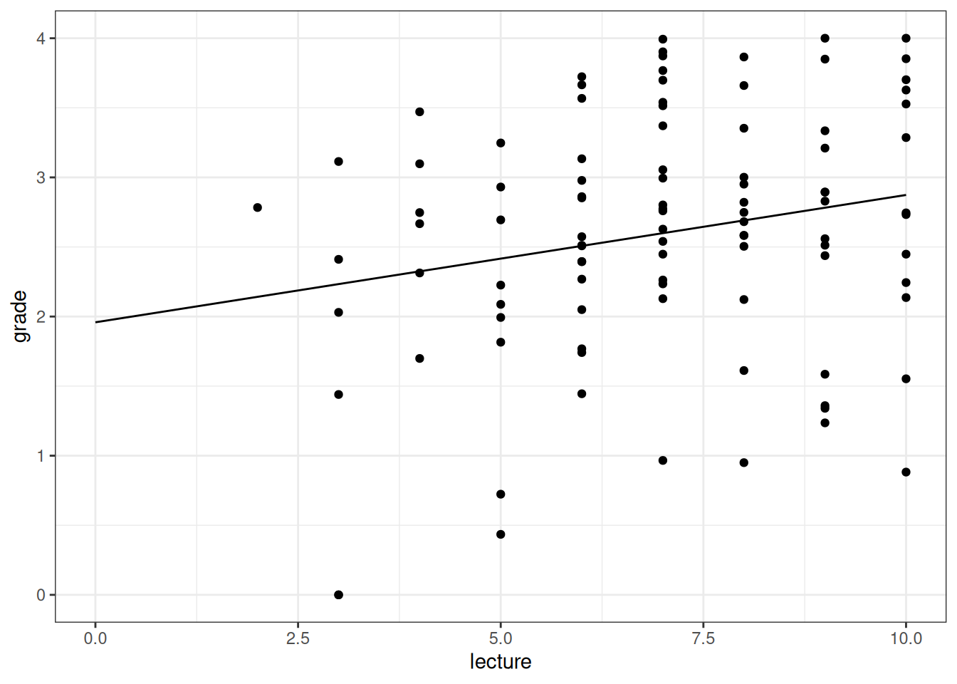

Figure 3.1: Partial effect of 'lecture' on grade, with nclicks at its mean value.

Partial effect plots only make sense when there are no interactions in the model between the focal predictor and any other predictor.

The reason is that when there are interactions, the partial effect of focal predictor $X_i$ will differ across the values of the other variables it interacts with.

Now can you visualize the partial effect of nclicks on grade?

See the solution at the bottom of the page.

3.1.5 Standardizing coefficients

One kind of question that we often use multiple regression to address is, Which predictors matter most in predicting Y?

Now, you can't just read off the $\hat{\beta}$ values and choose the one with the largest absolute value, because the predictors are all on different scales. To answer this question, you need to center and scale the predictors.

Remember $z$ scores?

\[ z = \frac{X - \mu_x}{\sigma_x} \]

A $z$ score represents the distance of a score $X$ from the sample mean ($\mu_x$) in standard deviation units ($\sigma_x$). So a $z$ score of 1 means that the score is one standard deviation about the mean; a $z$-score of -2.5 means 2.5 standard deviations below the mean. $Z$-scores give us a way of comparing things that come from different populations by calibrating them to the standard normal distribution (a distribution with a mean of 0 and a standard deviation of 1).

So we re-scale our predictors by converting them to $z$-scores. This is easy enough to do.

grades2 <- grades %>%
  mutate(lecture_c = (lecture - mean(lecture)) / sd(lecture),
         nclicks_c = (nclicks - mean(nclicks)) / sd(nclicks))

grades2

## # A tibble: 100 × 6
##    grade   GPA lecture nclicks lecture_c nclicks_c
##    <dbl> <dbl>   <int>   <int>     <dbl>     <dbl>
##  1  2.40 1.13        6      88  -0.484     -0.666 
##  2  3.67 0.971       6      96  -0.484     -0.150 
##  3  2.85 3.34        6     123  -0.484      1.59  
##  4  1.36 2.76        9      99   0.982      0.0439
##  5  2.31 1.02        4      66  -1.46      -2.09  
##  6  2.58 0.841       8      99   0.493      0.0439
##  7  2.69 4           5      86  -0.972     -0.796 
##  8  3.05 2.29        7     118   0.00488    1.27  
##  9  3.21 3.39        9      98   0.982     -0.0207
## 10  2.24 3.27       10     115   1.47       1.08  
## # ℹ 90 more rows

Now let's re-fit the model using the centered and scaled predictors.

my_model_scaled <- lm(grade ~ lecture_c + nclicks_c, grades2)

summary(my_model_scaled)

## 
## Call:
## lm(formula = grade ~ lecture_c + nclicks_c, data = grades2)
## 
## Residuals:
##      Min       1Q   Median       3Q      Max 
## -2.21653 -0.40603  0.02267  0.60720  1.38558 
## 
## Coefficients:
##             Estimate Std. Error t value Pr(>|t|)    
## (Intercept)  2.59839    0.08692  29.895   <2e-16 ***
## lecture_c    0.18734    0.09370   1.999   0.0484 *  
## nclicks_c    0.07823    0.09370   0.835   0.4058    
## ---
## Signif. codes:  0 '***' 0.001 '**' 0.01 '*' 0.05 '.' 0.1 ' ' 1
## 
## Residual standard error: 0.8692 on 97 degrees of freedom
## Multiple R-squared:  0.06543,    Adjusted R-squared:  0.04616 
## F-statistic: 3.395 on 2 and 97 DF,  p-value: 0.03756

This tells us that lecture_c has a relatively larger influence; for each standard deviation increase in this variable, grade increases by about 0.19.

Another common approach to standardization involves standardizing the response variable as well as the predictors, i.e., $z$-scoring the $Y$ values as well as the $X$ values. The relative rank order of the regression coefficients will be the same under this approach. The main difference would be that the coefficients will be expressed in standard deviation ($SD$) units of the response variable, rather than in raw units.

Multicollinearity and its discontents

In discussions about multiple regression you may hear concerns expressed about "multicollinearity", which is a fancy way of referring to the existence of intercorrelations among the predictor variables. This is only a potential problem insofar as it potentially affects the interpretation of the effects of individual predictor variables. When predictor variables are correlated, $\beta$ values can change depending upon which predictors are included or excluded from the model, sometimes even changing signs. The key things to keep in mind about this are:

correlated predictors are probably unavoidable in observational studies;
regression does not assume that your predictor variables are independent from one another (in other words, finding correlations amongst your predictors is not itself a reason to question your model);
when strong correlations are present, use caution in interpreting individual regression coefficients;
there is no known "remedy" for it, nor is it clear that any such remedy is desireable, and many so-called remedies do more harm than good.

For more information and guidance, see (Vanhove, 2021).

3.1.6 Model comparison

Another common kind of question multiple regression is also used to address is of the form: Does some predictor or set of predictors of interest significantly impact my response variable over and above the effects of some control variables?

For example, we saw above that the model including lecture and nclicks was statistically significant, $F(2, 97) = 3.395$, $p = 0.038$.

The null hypothesis for a regression model with $m$ predictors is

\[H_0: \beta_1 = \beta_2 = \ldots = \beta_m = 0;\]

in other words, that all of the coefficients (except the intercept) are zero. If the null hypothesis is true, then the null model

\[Y_i = \beta_0\]

gives just as good of a prediction as the model including all of the predictors and their coefficients. In other words, your best prediction for $Y$ is just its mean ($\mu_y$); the $X$ variables are irrelevant. We rejected this null hypothesis, which implies that we can do better by including our two predictors, lecture and nclicks.

But you might ask: maybe its the case that better students get better grades, and the relationship between lecture, nclicks, and grade is just mediated by student quality. After all, better students are more likely to go to lecture and download the materials. So we can ask, are attendance and downloads associated with better grades above and beyond student ability, as measured by GPA?

The way we can test this hypothesis is by using model comparison. The logic is as follows. First, estimate a model containing any control predictors but excluding the focal predictors of interest. Second, estimate a model containing the control predictors as well as the focal predictors. Finally, compare the two models, to see if there is any statistically significant gain by including the predictors.

Here is how you do this:

m1 <- lm(grade ~ GPA, grades) # control model
m2 <- lm(grade ~ GPA + lecture + nclicks, grades) # bigger model

anova(m1, m2)

## Analysis of Variance Table
## 
## Model 1: grade ~ GPA
## Model 2: grade ~ GPA + lecture + nclicks
##   Res.Df    RSS Df Sum of Sq      F Pr(>F)
## 1     98 73.528                           
## 2     96 71.578  2    1.9499 1.3076 0.2752

The null hypothesis is that we are just as good predicting grade from GPA as we are predicting it from GPA plus lecture and nclicks. We will reject the null if adding these two variables leads to a substantial enough reduction in the residual sums of squares (RSS); i.e., if they explain away enough residual variance.

We see that this is not the case: $F(2, 96 ) = 1.308$, $p = 0.275$. So we don't have evidence that lecture attendance and downloading the online materials is associated with better grades above and beyond student ability, as measured by GPA.

3.2 Dealing with categorical predictors

A regression formula characterizes the response variable as the sum of weighted predictors. What if one of the predictors is categorical (e.g., representing groups such as "rural" or "urban") rather than numeric? Many variables are nominal: a categorical variable containing names, for which there is no inherent ordering among the levels of the variable. Pet ownership (cat, dog, ferret) is a nominal variable; preferences aside, owning a cat is not greater than owning a dog, and owning a dog is not greater than owning a ferret.

Representing nominal data using numeric predictors

Representing a nominal variable with $k$ levels in a regression model requires $k-1$ numeric predictors; for instance, if you have four levels, you need three predictors. Most numerical coding schemes require that you choose one of these $k$ levels as a baseline level. Each of your $k-1$ variables contrasts one of the other levels level with the baseline.

Example: You have a variable, pet_type with three levels (cat, dog, ferret).

You choose cat as the baseline, and create two numeric predictor variables:

dog_v_cat to encode the contrast between dog and cat, and
ferret_v_cat to encode the contrast between ferret and cat.

Nominal variables are typically represented in a data frame as type character or factor.

The difference between a character and a factor variable is that factors contain information about the levels and their order, while character vectors lack this information.

When you specify a model using the R formula syntax, R will check the data types of the predictors on the right hand side of the formula. For example, if your model regresses income on pet_type (e.g., income ~ pet_type), R checks the data type of pet_type.

For any variable of type character or factor, R will implicitly create a numeric predictor (or a set of predictors) to represent that variable in the model. There are different schemes available for creating numeric representations of nominal variables. The default in R is to use dummy (or 'treatment') coding (see below). Unfortunately, this default is unsuitable for many types of study designs in psychology, so I am going to recommend that you learn how to code your own predictor variables "by hand," and that you make a habit of doing so.

Don't represent levels of a categorical variable with numbers!

In the above example, we had a variable pet_type with levels cat, dog, and ferret. Sometimes people represent the levels of a nominal variable with numbers, like so:

1 for cat,
2 for dog,
3 for ferret.

This is a bad idea.

First, the labeling is arbitrary and opaque and anyone attempting to use your data would not know which number goes with which category (and you could also forget!).

Even worse, if you were to put this variable in as a predictor in a regression model, R would have no way of knowing your intention to use 1, 2, and 3 as arbitrary labels for groups, and would instead assume that pet_type is a measurement for which dogs are 1 unit greater than cats, and ferrets are 2 units greater than cats and 1 unit greater than dogs, which is nonsense!

It is far too easy to make this mistake, and difficult to catch if authors do not share their data and code. In 2016, a paper on religious affiliation and altruism in children that was published in Current Biology had to be retracted for just this kind of mistake.

So, don't represent the levels of a nominal variable with numbers, except of course when you deliberately create predictor variables encoding the $k-1$ contrasts needed to properly represent a nominal variable in a regression model.

3.2.1 Dummy (a.k.a. "treatment") coding

For a nominal variable with only two levels, choose one level as baseline, and create a new variable that is 0 whenever the level is baseline and 1 when it is the other level. The choice of baseline is arbitrary, and will affect only whether the coefficient is positive or negative, but not its magnitude, its standard error nor the associated p-value.

To illustrate, let's gin up some fake data with a single two level categorical predictor.

fake_data <- tibble(Y = rnorm(10),
                    group = rep(c("A", "B"), each = 5))

fake_data

## # A tibble: 10 × 2
##         Y group
##     <dbl> <chr>
##  1  0.776 A    
##  2  0.175 A    
##  3 -0.466 A    
##  4 -1.40  A    
##  5 -0.498 A    
##  6  0.536 B    
##  7  0.527 B    
##  8 -2.06  B    
##  9 -0.894 B    
## 10 -1.22  B

Now let's add a new variable, group_d, which is the dummy coded group variable. We will use the dplyr::if_else() function to define the new column.

fake_data2 <- fake_data %>%
  mutate(group_d = if_else(group == "B", 1, 0))

fake_data2

## # A tibble: 10 × 3
##         Y group group_d
##     <dbl> <chr>   <dbl>
##  1  0.776 A           0
##  2  0.175 A           0
##  3 -0.466 A           0
##  4 -1.40  A           0
##  5 -0.498 A           0
##  6  0.536 B           1
##  7  0.527 B           1
##  8 -2.06  B           1
##  9 -0.894 B           1
## 10 -1.22  B           1

Now we just run it as a regular regression model.

summary(lm(Y ~ group_d, fake_data2))

## 
## Call:
## lm(formula = Y ~ group_d, data = fake_data2)
## 
## Residuals:
##     Min      1Q  Median      3Q     Max 
## -1.4380 -0.5167 -0.2001  0.9078  1.1582 
## 
## Coefficients:
##             Estimate Std. Error t value Pr(>|t|)
## (Intercept)  -0.2816     0.4420  -0.637    0.542
## group_d      -0.3408     0.6251  -0.545    0.601
## 
## Residual standard error: 0.9883 on 8 degrees of freedom
## Multiple R-squared:  0.03582,    Adjusted R-squared:  -0.0847 
## F-statistic: 0.2972 on 1 and 8 DF,  p-value: 0.6005

Let's reverse the coding. We get the same result, just the sign is different.

fake_data3 <- fake_data %>%
  mutate(group_d = if_else(group == "A", 1, 0))

summary(lm(Y ~ group_d, fake_data3))

## 
## Call:
## lm(formula = Y ~ group_d, data = fake_data3)
## 
## Residuals:
##     Min      1Q  Median      3Q     Max 
## -1.4380 -0.5167 -0.2001  0.9078  1.1582 
## 
## Coefficients:
##             Estimate Std. Error t value Pr(>|t|)
## (Intercept)  -0.6224     0.4420  -1.408    0.197
## group_d       0.3408     0.6251   0.545    0.601
## 
## Residual standard error: 0.9883 on 8 degrees of freedom
## Multiple R-squared:  0.03582,    Adjusted R-squared:  -0.0847 
## F-statistic: 0.2972 on 1 and 8 DF,  p-value: 0.6005

The interpretation of the intercept is the estimated mean for the group coded as zero. You can see by plugging in zero for X in the prediction formula below. Thus, $\beta_1$ can be interpreted as the difference between the mean for the baseline group and the group coded as 1.

\[\hat{Y_i} = \hat{\beta}_0 + \hat{\beta}_1 X_i \]

Note that if we just put the character variable group as a predictor in the model, R will automatically create a dummy variable (or variables) for us as needed.

lm(Y ~ group, fake_data) %>%
  summary()

## 
## Call:
## lm(formula = Y ~ group, data = fake_data)
## 
## Residuals:
##     Min      1Q  Median      3Q     Max 
## -1.4380 -0.5167 -0.2001  0.9078  1.1582 
## 
## Coefficients:
##             Estimate Std. Error t value Pr(>|t|)
## (Intercept)  -0.2816     0.4420  -0.637    0.542
## groupB       -0.3408     0.6251  -0.545    0.601
## 
## Residual standard error: 0.9883 on 8 degrees of freedom
## Multiple R-squared:  0.03582,    Adjusted R-squared:  -0.0847 
## F-statistic: 0.2972 on 1 and 8 DF,  p-value: 0.6005

The lm() function examines group and figures out the unique levels of the variable, which in this case are A and B. It then chooses as baseline the level that comes first alphabetically, and encodes the contrast between the other level (B) and the baseline level (A). (In the case where group has been defined as a factor, the baseline level is the first element of levels(fake_data$group)).

This new variable that it created shows up with the name groupB in the output.

3.2.2 Dummy coding when $k > 2$

When a nominal predictor variable has more than two levels ($k > 2$), one numeric predictor is no longer sufficient; we need $k-1$ predictors. If the nominal predictor has four levels, we'll need to define three predictors. Let's simulate some data to work with, season_wt, which represents a person's bodyweight (in kg) over the four seasons of the year.

season_wt <- tibble(season = rep(c("winter", "spring", "summer", "fall"),
                                 each = 5),
                    bodyweight_kg = c(rnorm(5, 105, 3),
                                      rnorm(5, 103, 3),
                                      rnorm(5, 101, 3),
                                      rnorm(5, 102.5, 3)))

season_wt

## # A tibble: 20 × 2
##    season bodyweight_kg
##    <chr>          <dbl>
##  1 winter          107.
##  2 winter          105.
##  3 winter          106.
##  4 winter          107.
##  5 winter          105.
##  6 spring          101.
##  7 spring          102.
##  8 spring          103.
##  9 spring          108.
## 10 spring          105.
## 11 summer          106.
## 12 summer          102.
## 13 summer          100.
## 14 summer          103.
## 15 summer          102.
## 16 fall            107.
## 17 fall            105.
## 18 fall            103.
## 19 fall            101.
## 20 fall            101.

Now let's add three predictors to code the variable season. Try it out and see if you can figure out how it works.

## baseline value is 'winter'
season_wt2 <- season_wt %>%
  mutate(spring_v_winter = if_else(season == "spring", 1, 0),
         summer_v_winter = if_else(season == "summer", 1, 0),
         fall_v_winter = if_else(season == "fall", 1, 0))

season_wt2

## # A tibble: 20 × 5
##    season bodyweight_kg spring_v_winter summer_v_winter fall_v_winter
##    <chr>          <dbl>           <dbl>           <dbl>         <dbl>
##  1 winter          107.               0               0             0
##  2 winter          105.               0               0             0
##  3 winter          106.               0               0             0
##  4 winter          107.               0               0             0
##  5 winter          105.               0               0             0
##  6 spring          101.               1               0             0
##  7 spring          102.               1               0             0
##  8 spring          103.               1               0             0
##  9 spring          108.               1               0             0
## 10 spring          105.               1               0             0
## 11 summer          106.               0               1             0
## 12 summer          102.               0               1             0
## 13 summer          100.               0               1             0
## 14 summer          103.               0               1             0
## 15 summer          102.               0               1             0
## 16 fall            107.               0               0             1
## 17 fall            105.               0               0             1
## 18 fall            103.               0               0             1
## 19 fall            101.               0               0             1
## 20 fall            101.               0               0             1

Reminder: Always look at your data

Whenever you write code that potentially changes your data, you should double check that the code works as intended by looking at your data. This is especially the case when you are hand-coding nominal variables for use in regression, because sometimes the code will be wrong, but won't throw an error.

Consider the code chunk above, where we defined three contrasts to represent the nominal variable season, with winter as our baseline.

What would happen if you accidently misspelled one of the levels (summre for summer) and didn't notice?

season_wt3 <- season_wt %>%
  mutate(spring_v_winter = if_else(season == "spring", 1, 0),
         summer_v_winter = if_else(season == "summre", 1, 0),
         fall_v_winter = if_else(season == "fall", 1, 0))

While the above code chunk runs, we get confusing output when we run the regression; namely, the coefficent for summer_v_winter is NA (not available).

lm(bodyweight_kg ~ spring_v_winter + summer_v_winter + fall_v_winter,
   season_wt3)

## 
## Call:
## lm(formula = bodyweight_kg ~ spring_v_winter + summer_v_winter + 
##     fall_v_winter, data = season_wt3)
## 
## Coefficients:
##     (Intercept)  spring_v_winter  summer_v_winter    fall_v_winter  
##        104.2673          -0.3439               NA          -0.9552

What happened? Let's look at the data to find out. We will use distinct to find the distinct combinations of our original variable season with the three variables we created (see ?dplyr::distinct for details).

season_wt3 %>%
  distinct(season, spring_v_winter, summer_v_winter, fall_v_winter)

## # A tibble: 4 × 4
##   season spring_v_winter summer_v_winter fall_v_winter
##   <chr>            <dbl>           <dbl>         <dbl>
## 1 winter               0               0             0
## 2 spring               1               0             0
## 3 summer               0               0             0
## 4 fall                 0               0             1

Because of our misspelling, the predictor summer_v_winter is not 1 when season == "summer"; instead, it is always zero. The if_else() above literally says 'set summer_v_winter to 1 if season == "summre", otherwise 0'. Of course, season is never equal to summre, because summre is a typo. We could have caught this easily by running the above check with distinct(). Get in the habit of doing this when you create your own numeric predictors.

A closer look at R's defaults

If you've ever used point-and-click statistical software like SPSS, you probably never had to learn about coding categorical predictors. Normally, the software recognizes when a predictor is categorical and, behind the scenes, it takes care of recoding it into a numerical predictor. R is no different: if you supply a predictor of type character or factor to a linear modeling function, it will create numerical dummy-coded predictors for you, as shown in the code below.

lm(bodyweight_kg ~ season, season_wt) %>%
  summary()

## 
## Call:
## lm(formula = bodyweight_kg ~ season, data = season_wt)
## 
## Residuals:
##     Min      1Q  Median      3Q     Max 
## -2.7820 -1.1927 -0.6222  0.9015  3.8698 
## 
## Coefficients:
##              Estimate Std. Error t value Pr(>|t|)    
## (Intercept)  103.3121     0.9597 107.648   <2e-16 ***
## seasonspring   0.6114     1.3572   0.450   0.6584    
## seasonsummer  -0.7879     1.3572  -0.581   0.5696    
## seasonwinter   2.6984     1.3572   1.988   0.0642 .  
## ---
## Signif. codes:  0 '***' 0.001 '**' 0.01 '*' 0.05 '.' 0.1 ' ' 1
## 
## Residual standard error: 2.146 on 16 degrees of freedom
## Multiple R-squared:  0.3121, Adjusted R-squared:  0.1831 
## F-statistic:  2.42 on 3 and 16 DF,  p-value: 0.104

Here, R implicitly creates three dummy variables to code the four levels of season, called seasonspring, seasonsummer and seasonwinter. The unmentioned season, fall, has been chosen as baseline because it comes earliest in the alphabet. These three predictors have the following values:

seasonspring: 1 if spring, 0 otherwise;
seasonsummer: 1 if summer, 0 otherwise;
seasonwinter: 1 if winter, 0 otherwise.

This seems like a handy thing to have R do for us, but dangers lurk in relying on the default. We'll learn more about these dangers in the next chapter when we talk about interactions.

3.3 Equivalence between multiple regression and one-way ANOVA

If we wanted to see whether our bodyweight varies over season, we could do a one way ANOVA on season_wt2 like so.

## make season into a factor with baseline level 'winter'
season_wt3 <- season_wt2 %>%
  mutate(season = factor(season, levels = c("winter", "spring",
                                            "summer", "fall")))

my_anova <- aov(bodyweight_kg ~ season, season_wt3)
summary(my_anova)

##             Df Sum Sq Mean Sq F value Pr(>F)
## season       3  33.43  11.143    2.42  0.104
## Residuals   16  73.68   4.605

OK, now can we replicate that result using the regression model below?

\[Y_i = \beta_0 + \beta_1 X_{1i} + \beta_2 X_{2i} + \beta_3 X_{3i} + e_i\]

summary(lm(bodyweight_kg ~ spring_v_winter +
             summer_v_winter + fall_v_winter,
           season_wt2))

## 
## Call:
## lm(formula = bodyweight_kg ~ spring_v_winter + summer_v_winter + 
##     fall_v_winter, data = season_wt2)
## 
## Residuals:
##     Min      1Q  Median      3Q     Max 
## -2.7820 -1.1927 -0.6222  0.9015  3.8698 
## 
## Coefficients:
##                 Estimate Std. Error t value Pr(>|t|)    
## (Intercept)     106.0105     0.9597 110.460   <2e-16 ***
## spring_v_winter  -2.0870     1.3572  -1.538   0.1437    
## summer_v_winter  -3.4863     1.3572  -2.569   0.0206 *  
## fall_v_winter    -2.6984     1.3572  -1.988   0.0642 .  
## ---
## Signif. codes:  0 '***' 0.001 '**' 0.01 '*' 0.05 '.' 0.1 ' ' 1
## 
## Residual standard error: 2.146 on 16 degrees of freedom
## Multiple R-squared:  0.3121, Adjusted R-squared:  0.1831 
## F-statistic:  2.42 on 3 and 16 DF,  p-value: 0.104

Note that the $F$ values and $p$ values are identical for the two methods!

3.4 Solutions to exercises

First create a tibble with new predictors. We might also want to know the range of values that nclicks varies over.

lecture_mean <- grades %>% pull(lecture) %>% mean()
min_nclicks <- grades %>% pull(nclicks) %>% min()
max_nclicks <- grades %>% pull(nclicks) %>% max()

## new data for prediction
new_nclicks <- tibble(lecture = lecture_mean,
                      nclicks = min_nclicks:max_nclicks)

## add the predicted value to new_lecture
new_nclicks2 <- new_nclicks %>%
  mutate(grade = predict(my_model, new_nclicks))

new_nclicks2

## # A tibble: 76 × 3
##    lecture nclicks grade
##      <dbl>   <int> <dbl>
##  1    6.99      54  2.37
##  2    6.99      55  2.38
##  3    6.99      56  2.38
##  4    6.99      57  2.39
##  5    6.99      58  2.39
##  6    6.99      59  2.40
##  7    6.99      60  2.40
##  8    6.99      61  2.41
##  9    6.99      62  2.41
## 10    6.99      63  2.42
## # ℹ 66 more rows

Now plot.

ggplot(grades, aes(nclicks, grade)) +
  geom_point() +
  geom_line(data = new_nclicks2)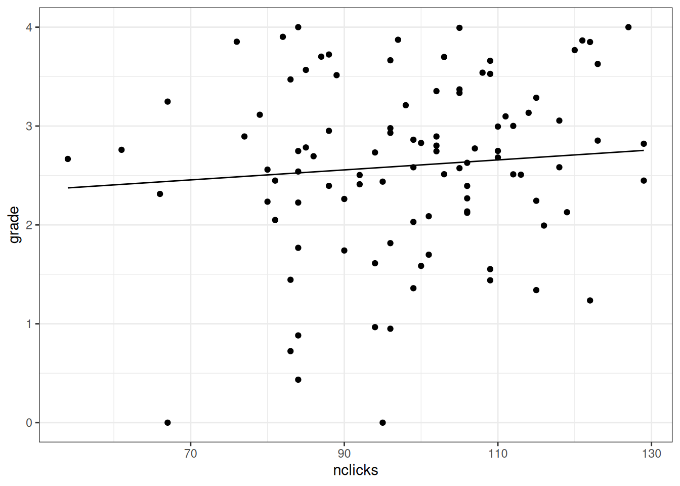

Figure 3.2: Partial effect plot of nclicks on grade.

2 Correlation and regression

4 Interactions

Learning Statistical Models Through Simulation in R

3 Multiple regression

3.1 An example: How to get a good grade in statistics

3.1.1 Data import and visualization

3.1.2 Estimation and interpretation

3.1.3 Predictions from the linear model using `predict()`

3.1.4 Visualizing partial effects

3.1.5 Standardizing coefficients

3.1.6 Model comparison

3.2 Dealing with categorical predictors

3.2.1 Dummy (a.k.a. "treatment") coding

3.2.2 Dummy coding when \(k > 2\)

3.3 Equivalence between multiple regression and one-way ANOVA

3.4 Solutions to exercises

3 Multiple regression

3.1 An example: How to get a good grade in statistics

3.1.1 Data import and visualization

3.1.2 Estimation and interpretation

3.1.3 Predictions from the linear model using predict()

3.1.4 Visualizing partial effects

3.1.5 Standardizing coefficients

3.1.6 Model comparison

3.2 Dealing with categorical predictors

3.2.1 Dummy (a.k.a. "treatment") coding

3.2.2 Dummy coding when \(k > 2\)

3.3 Equivalence between multiple regression and one-way ANOVA

3.4 Solutions to exercises

3.1.3 Predictions from the linear model using `predict()`