Chapter 3 Multiple regression
You are reading an old version of this textbook.
General model for single-level data with \(m\) predictors:
\[ Y_i = \beta_0 + \beta_1 X_{1i} + \beta_2 X_{2i} + \ldots + \beta_m X_{mi} + e_i \]
The individual \(X_{hi}\) variables can be any combination of continuous and/or categorical predictors, including interactions among variables.
The \(\beta\) values are referred to as regression coefficients. Each \(\beta_h\) is interpreted as the partial effect of \(\beta_h\) holding constant all other predictor variables. If you have \(m\) predictor variables, you have \(m+1\) regression coefficients: one for the intercept, and one for each predictor.
Although discussions of multiple regression are common in statistical textbooks, you will rarely be able to apply the exact model above. This is because the above model assumes single-level data, whereas most psychological data is multi-level. However, the fundamentals are the same for both types of datasets, so it is worthwhile learning them for the simpler case first.
3.1 An example: How to get a good grade in statistics
Let’s look at some (made up, but realistic) data to see how we can use multiple regression to answer various study questions. In this hypothetical study, you have a dataset for 100 statistics students, which includes their final course grade (grade), the number of lectures each student attended (lecture, an integer ranging from 0-10), how many times each student clicked to download online materials (nclicks) and each student’s grade point average prior to taking the course, GPA, which ranges from 0 (fail) to 4 (highest possible grade).
3.1.1 Data import and visualization
Let’s load in the data grades.csv and have a look.
library("corrr") # correlation matrices
library("tidyverse")

grades <- read_csv("data/grades.csv", col_types = "ddii")

grades
## # A tibble: 100 x 4
## grade GPA lecture nclicks
## <dbl> <dbl> <int> <int>
## 1 2.40 1.13 6 88
## 2 3.67 0.971 6 96
## 3 2.85 3.34 6 123
## 4 1.36 2.76 9 99
## 5 2.31 1.02 4 66
## 6 2.58 0.841 8 99
## 7 2.69 4 5 86
## 8 3.05 2.29 7 118
## 9 3.21 3.39 9 98
## 10 2.24 3.27 10 115
## # … with 90 more rowsFirst let’s look at all the pairwise correlations.
##
## Correlation method: 'pearson'
## Missing treated using: 'pairwise.complete.obs'
## term grade GPA lecture nclicks
## 1 grade
## 2 GPA .25
## 3 lecture .24 .44
## 4 nclicks .16 .30 .36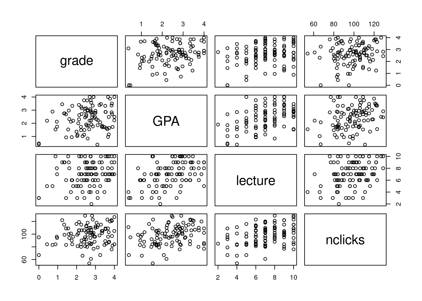
Figure 2.2: All pairwise relationships in the grades dataset.
3.1.2 Estimation and interpretation
To estimate the regression coefficients (the \(\beta\)s), we will use the lm() function. For a GLM with \(m\) predictors:
\[ Y_i = \beta_0 + \beta_1 X_{1i} + \beta_2 X_{2i} + \ldots + \beta_m X_{mi} + e_i \]
The call to base R’s lm() is
lm(Y ~ X1 + X2 + ... + Xm, data)
The Y variable is your response variable, and the X variables are the predictor variables. Note that you don’t need to explicitly specify the intercept or residual terms; those are included by default.
For the current data, let’s predict grade from lecture and nclicks.
##
## Call:
## lm(formula = grade ~ lecture + nclicks, data = grades)
##
## Residuals:
##      Min       1Q   Median       3Q      Max
## -2.21653 -0.40603  0.02267  0.60720  1.38558
##
## Coefficients:
##             Estimate Std. Error t value Pr(>|t|)
## (Intercept) 1.462037   0.571124   2.560   0.0120 *
## lecture     0.091501   0.045766   1.999   0.0484 *
## nclicks     0.005052   0.006051   0.835   0.4058
## ---
## Signif. codes:  0 '***' 0.001 '**' 0.01 '*' 0.05 '.' 0.1 ' ' 1
##
## Residual standard error: 0.8692 on 97 degrees of freedom
## Multiple R-squared:  0.06543,    Adjusted R-squared:  0.04616
## F-statistic: 3.395 on 2 and 97 DF,  p-value: 0.03756
We’ll often write the parameter symbol with a little hat on top to make clear that we are dealing with estimates from the sample rather than the (unknown) true population values. From above:
- \(\hat{\beta}_0\) = 1.46
- \(\hat{\beta}_1\) = 0.09
- \(\hat{\beta}_2\) = 0.01
This tells us that a person’s predicted grade is related to their lecture attendance and download rate by the following formula:
grade = 1.46 + 0.09 \(\times\) lecture + 0.01 \(\times\) nclicks
Because \(\hat{\beta}_1\) and \(\hat{\beta}_2\) are both positive, we know that higher values of lecture and nclicks are associated with higher grades.
So if you were asked, what grade would you predict for a student who attends 3 lectures and downloaded 70 times, you could easily figure that out by substituting the appropriate values.
grade = 1.46 + 0.09 \(\times\) 3 + 0.01 \(\times\) 70
which equals
grade = 1.46 + 0.27 + 0.7
and reduces to
grade = 2.43
3.1.3 Predictions from the linear model using predict()
If we want to predict response values for new predictor values, we can use the predict() function in base R.
predict() takes two main arguments. The first argument is a fitted model object (i.e., my_model from above) and the second is a data frame (or tibble) containing new values for the predictors.
You need to include all of the predictor variables in the new table. You’ll get an error message if your tibble is missing any predictors. You also need to make sure that the variable names in the new table exactly match the variable names in the model.
Let’s create a tibble with new values and try it out.
## a 'tribble' is a way to make a tibble by rows,
## rather than by columns. This is sometimes useful
new_data <- tribble(~lecture, ~nclicks,
                    3, 70,
                    10, 130,
                    0, 20,
                    5, 100)
The tribble() function provides a way to build a tibble row by row, whereas with tibble() the table is built column by column.
The first row of the tribble() contains the column names, each preceded by a tilde (~).
This is sometimes easier to read than doing it row by row, although the result is the same. Consider that we could have made the above table using
Now that we’ve created our table new_data, we just pass it to predict() and it will return a vector with the predictions for \(Y\) (grade).
##        1        2        3        4
## 2.090214 3.033869 1.563087 2.424790
That’s great, but maybe we want to line it up with the predictor values. We can do this by just adding it as a new column to new_data.
## # A tibble: 4 x 3
##   lecture nclicks predicted_grade
##     <dbl>   <dbl>           <dbl>
## 1       3      70            2.09
## 2      10     130            3.03
## 3       0      20            1.56
## 4       5     100            2.42
Want to see more options for predict()? Check the help at ?predict.lm.
3.1.4 Visualizing partial effects
As noted above the parameter estimates for each regression coefficient tell us about the partial effect of that variable; it’s effect holding all of the others constant. Is there a way to visualize this partial effect? Yes, you can do this using the predict() function, by making a table with varying values for the focal predictor, while filling in all of the other predictors with their mean values.
For example, let’s visualize the partial effect of lecture on grade holding nclicks constant at its mean value.
nclicks_mean <- grades %>% pull(nclicks) %>% mean()

## new data for prediction
new_lecture <- tibble(lecture = 0:10,
                      nclicks = nclicks_mean)

## add the predicted value to new_lecture
new_lecture2 <- new_lecture %>%
  mutate(grade = predict(my_model, new_lecture))

new_lecture2
## # A tibble: 11 x 3
## lecture nclicks grade
## <int> <dbl> <dbl>
## 1 0 98.3 1.96
## 2 1 98.3 2.05
## 3 2 98.3 2.14
## 4 3 98.3 2.23
## 5 4 98.3 2.32
## 6 5 98.3 2.42
## 7 6 98.3 2.51
## 8 7 98.3 2.60
## 9 8 98.3 2.69
## 10 9 98.3 2.78
## 11 10 98.3 2.87Now let’s plot.
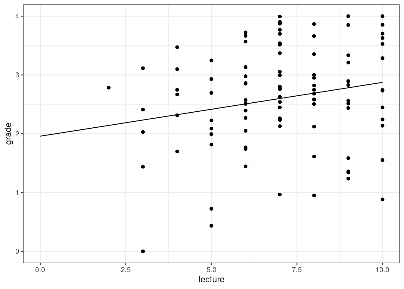
Figure 3.1: Partial effect of ‘lecture’ on grade, with nclicks at its mean value.
Partial effect plots only make sense when there are no interactions in the model between the focal predictor and any other predictor.
The reason is that when there are interactions, the partial effect of focal predictor \(X_i\) will differ across the values of the other variables it interacts with.
Now can you visualize the partial effect of nclicks on grade?
See the solution at the bottom of the page.
3.1.5 Standardizing coefficients
One kind of question that we often use multiple regression to address is, Which predictors matter most in predicting Y?
Now, you can’t just read off the \(\hat{\beta}\) values and choose the one with the largest absolute value, because the predictors are all on different scales. To answer this question, you need to center and scale the predictors.
Remember \(z\) scores?
\[ z = \frac{X - \mu_x}{\sigma_x} \]
A \(z\) score represents the distance of a score \(X\) from the sample mean (\(\mu_x\)) in standard deviation units (\(\sigma_x\)). So a \(z\) score of 1 means that the score is one standard deviation about the mean; a \(z\)-score of -2.5 means 2.5 standard deviations below the mean. \(Z\)-scores give us a way of comparing things that come from different populations by calibrating them to the standard normal distribution (a distribution with a mean of 0 and a standard deviation of 1).
So we re-scale our predictors by converting them to \(z\)-scores. This is easy enough to do.
grades2 <- grades %>%
  mutate(lecture_c = (lecture - mean(lecture)) / sd(lecture),
         nclicks_c = (nclicks - mean(nclicks)) / sd(nclicks))

grades2
## # A tibble: 100 x 6
## grade GPA lecture nclicks lecture_c nclicks_c
## <dbl> <dbl> <int> <int> <dbl> <dbl>
## 1 2.40 1.13 6 88 -0.484 -0.666
## 2 3.67 0.971 6 96 -0.484 -0.150
## 3 2.85 3.34 6 123 -0.484 1.59
## 4 1.36 2.76 9 99 0.982 0.0439
## 5 2.31 1.02 4 66 -1.46 -2.09
## 6 2.58 0.841 8 99 0.493 0.0439
## 7 2.69 4 5 86 -0.972 -0.796
## 8 3.05 2.29 7 118 0.00488 1.27
## 9 3.21 3.39 9 98 0.982 -0.0207
## 10 2.24 3.27 10 115 1.47 1.08
## # … with 90 more rowsNow let’s re-fit the model using the centered and scaled predictors.
##
## Call:
## lm(formula = grade ~ lecture_c + nclicks_c, data = grades2)
##
## Residuals:
##      Min       1Q   Median       3Q      Max
## -2.21653 -0.40603  0.02267  0.60720  1.38558
##
## Coefficients:
##             Estimate Std. Error t value Pr(>|t|)
## (Intercept)  2.59839    0.08692  29.895   <2e-16 ***
## lecture_c    0.18734    0.09370   1.999   0.0484 *
## nclicks_c    0.07823    0.09370   0.835   0.4058
## ---
## Signif. codes:  0 '***' 0.001 '**' 0.01 '*' 0.05 '.' 0.1 ' ' 1
##
## Residual standard error: 0.8692 on 97 degrees of freedom
## Multiple R-squared:  0.06543,    Adjusted R-squared:  0.04616
## F-statistic: 3.395 on 2 and 97 DF,  p-value: 0.03756
This tells us that lecture_c has a relatively larger influence; for each standard deviation increase in this variable, grade increases by about 0.19.
3.1.6 Model comparison
Another common kind of question multiple regression is also used to address is of the form: Does some predictor or set of predictors of interest significantly impact my response variable over and above the effects of some control variables?
For example, we saw above that the model including lecture and nclicks was statistically significant,
\(F(2, 97) = 3.395\),
\(p = 0.038\).
The null hypothesis for a regression model with \(m\) predictors is
\[H_0: \beta_1 = \beta_2 = \ldots = \beta_m = 0;\]
in other words, that all of the coefficients (except the intercept) are zero. If the null hypothesis is true, then the null model
\[Y_i = \beta_0\]
gives just as good of a prediction as the model including all of the predictors and their coefficients. In other words, your best prediction for \(Y\) is just its mean (\(\mu_y\)); the \(X\) variables are irrelevant. We rejected this null hypothesis, which implies that we can do better by including our two predictors, lecture and nclicks.
But you might ask: maybe its the case that better students get better grades, and the relationship between lecture, nclicks, and grade is just mediated by student quality. After all, better students are more likely to go to lecture and download the materials. So we can ask, are attendance and downloads associated with better grades above and beyond student ability, as measured by GPA?
The way we can test this hypothesis is by using model comparison. The logic is as follows. First, estimate a model containing any control predictors but excluding the focal predictors of interest. Second, estimate a model containing the control predictors as well as the focal predictors. Finally, compare the two models, to see if there is any statistically significant gain by including the predictors.
Here is how you do this:
m1 <- lm(grade ~ GPA, grades) # control model
m2 <- lm(grade ~ GPA + lecture + nclicks, grades) # bigger model

anova(m1, m2)
## Analysis of Variance Table
##
## Model 1: grade ~ GPA
## Model 2: grade ~ GPA + lecture + nclicks
## Res.Df RSS Df Sum of Sq F Pr(>F)
## 1 98 73.528
## 2 96 71.578 2 1.9499 1.3076 0.2752The null hypothesis is that we are just as good predicting grade from GPA as we are predicting it from GPA plus lecture and nclicks. We will reject the null if adding these two variables leads to a substantial enough reduction in the residual sums of squares (RSS); i.e., if they explain away enough residual variance.
We see that this is not the case: \(F(2, 96 ) = 1.308\), \(p = 0.275\). So we don’t have evidence that lecture attendance and downloading the online materials is associated with better grades above and beyond student ability, as measured by GPA.
3.2 Dealing with categorical predictors
You can include categorical predictors in a regression model, but first you have to code them as numerical variables. There are a couple of important considerations here.
A nominal variable is a categorical variable for which there is no inherent ordering among the levels of the variable. Pet ownership (cat, dog, ferret) is a nominal variable; cat is not greater than dog and dog is not greater than ferret.
It is common to code nominal variables using numbers. However, you have to be very careful about using numerically-coded nominal variables in your models. If you have a number that is really just a nominal variable, make sure you define it as type factor() before entering it into the model. Otherwise, it will try to treat it as an actual number, and the results of your modeling will be garbage!
It is far too easy to make this mistake, and difficult to catch if authors do not share their data and code. In 2016, a paper on religious affiliation and altruism in children that was published in Current Biology had to be retracted for just this kind of mistake.
3.2.1 Dummy coding
For a factor with two levels, choose one level as zero and the other as one. The choice is arbitrary, and will affect the sign of the coefficient, but not its standard error or p-value. Here is some code that will do this. Note that if you have a predictor of type character or factor, R will automatically do that for you. We don’t want R to do this for reasons that will become apparent in the next lecture, so let’s learn how to make our own numeric predictor.
First, we gin up some fake data to use in our analysis.
## # A tibble: 10 x 2
##           Y group
##       <dbl> <chr>
##  1  1.32    A
##  2 -0.780   A
##  3  0.174   A
##  4  3.05    A
##  5  0.694   A
##  6  0.112   B
##  7  0.00135 B
##  8  0.691   B
##  9 -1.10    B
## 10  1.52    B
Now let’s add a new variable, group_d, which is the dummy coded group variable. We will use the dplyr::if_else() function to define the new column.
## # A tibble: 10 x 3
##           Y group group_d
##       <dbl> <chr>   <dbl>
##  1  1.32    A           0
##  2 -0.780   A           0
##  3  0.174   A           0
##  4  3.05    A           0
##  5  0.694   A           0
##  6  0.112   B           1
##  7  0.00135 B           1
##  8  0.691   B           1
##  9 -1.10    B           1
## 10  1.52    B           1
Now we just run it as a regular regression model.
##
## Call:
## lm(formula = Y ~ group_d, data = fake_data2)
##
## Residuals:
##     Min      1Q  Median      3Q     Max
## -1.6716 -0.5992 -0.1658  0.4409  2.1628
##
## Coefficients:
##             Estimate Std. Error t value Pr(>|t|)
## (Intercept)   0.8919     0.5455   1.635    0.141
## group_d      -0.6467     0.7715  -0.838    0.426
##
## Residual standard error: 1.22 on 8 degrees of freedom
## Multiple R-squared:  0.08075,    Adjusted R-squared:  -0.03416
## F-statistic: 0.7027 on 1 and 8 DF,  p-value: 0.4262
Note that if we reverse the coding we get the same result, just the sign is different.
fake_data3 <- fake_data %>%
  mutate(group_d = if_else(group == "A", 1, 0))

summary(lm(Y ~ group_d, fake_data3))
##
## Call:
## lm(formula = Y ~ group_d, data = fake_data3)
##
## Residuals:
## Min 1Q Median 3Q Max
## -1.6716 -0.5992 -0.1658 0.4409 2.1628
##
## Coefficients:
## Estimate Std. Error t value Pr(>|t|)
## (Intercept) 0.2452 0.5455 0.449 0.665
## group_d 0.6467 0.7715 0.838 0.426
##
## Residual standard error: 1.22 on 8 degrees of freedom
## Multiple R-squared: 0.08075, Adjusted R-squared: -0.03416
## F-statistic: 0.7027 on 1 and 8 DF, p-value: 0.4262The interpretation of the intercept is the estimated mean for the group coded as zero. You can see by plugging in zero for X in the prediction formula below. Thus, \(\beta_1\) can be interpreted as the difference between the mean for the baseline group and the group coded as 1.
\[\hat{Y_i} = \hat{\beta}_0 + \hat{\beta}_1 X_i \]
3.2.2 Dummy coding when \(k > 2\)
When the predictor variable is a factor with \(k\) levels where \(k>2\), we need \(k-1\) predictors to code that variable. So if the factor has 4 levels, we’ll need to define three predictors. Here is code to do that. Try it out and see if you can figure out how it works.
mydata <- tibble(season = rep(c("winter", "spring", "summer", "fall"), each = 5),
                 bodyweight_kg = c(rnorm(5, 105, 3),
                                   rnorm(5, 103, 3),
                                   rnorm(5, 101, 3),
                                   rnorm(5, 102.5, 3)))

mydata
## # A tibble: 20 x 2
## season bodyweight_kg
## <chr> <dbl>
## 1 winter 110.
## 2 winter 106.
## 3 winter 105.
## 4 winter 101.
## 5 winter 102.
## 6 spring 99.6
## 7 spring 99.6
## 8 spring 103.
## 9 spring 102.
## 10 spring 106.
## 11 summer 104.
## 12 summer 102.
## 13 summer 99.8
## 14 summer 102.
## 15 summer 104.
## 16 fall 99.7
## 17 fall 103.
## 18 fall 101.
## 19 fall 99.6
## 20 fall 97.6Now let’s add three predictors to code the variable season.
## baseline value is 'winter'
mydata2 <- mydata %>%
  mutate(V1 = if_else(season == "spring", 1, 0),
         V2 = if_else(season == "summer", 1, 0),
         V3 = if_else(season == "fall", 1, 0))

mydata2
## # A tibble: 20 x 5
## season bodyweight_kg V1 V2 V3
## <chr> <dbl> <dbl> <dbl> <dbl>
## 1 winter 110. 0 0 0
## 2 winter 106. 0 0 0
## 3 winter 105. 0 0 0
## 4 winter 101. 0 0 0
## 5 winter 102. 0 0 0
## 6 spring 99.6 1 0 0
## 7 spring 99.6 1 0 0
## 8 spring 103. 1 0 0
## 9 spring 102. 1 0 0
## 10 spring 106. 1 0 0
## 11 summer 104. 0 1 0
## 12 summer 102. 0 1 0
## 13 summer 99.8 0 1 0
## 14 summer 102. 0 1 0
## 15 summer 104. 0 1 0
## 16 fall 99.7 0 0 1
## 17 fall 103. 0 0 1
## 18 fall 101. 0 0 1
## 19 fall 99.6 0 0 1
## 20 fall 97.6 0 0 13.3 Equivalence between multiple regression and one-way ANOVA
If we wanted to see whether our bodyweight varies over season, we could do a one way ANOVA on mydata2 like so.
## make season into a factor with baseline level 'winter'
mydata3 <- mydata2 %>%
  mutate(season = factor(season, levels = c("winter", "spring", "summer", "fall")))

my_anova <- aov(bodyweight_kg ~ season, mydata3)
summary(my_anova)
## Df Sum Sq Mean Sq F value Pr(>F)
## season 3 55.92 18.639 3.076 0.0576 .
## Residuals 16 96.94 6.059
## ---
## Signif. codes: 0 '***' 0.001 '**' 0.01 '*' 0.05 '.' 0.1 ' ' 1OK, now can we replicate that result using the regression model below?
\[Y_i = \beta_0 + \beta_1 X_{1i} + \beta_2 X_{2i} + \beta_3 X_{3i} + e_i\]
##
## Call:
## lm(formula = bodyweight_kg ~ V1 + V2 + V3, data = mydata3)
##
## Residuals:
##     Min      1Q  Median      3Q     Max
## -3.4033 -2.3646  0.0264  1.0679  4.6606
##
## Coefficients:
##             Estimate Std. Error t value Pr(>|t|)
## (Intercept)  104.871      1.101  95.269  < 2e-16 ***
## V1            -2.906      1.557  -1.867  0.08036 .
## V2            -2.409      1.557  -1.548  0.14125
## V3            -4.682      1.557  -3.007  0.00835 **
## ---
## Signif. codes:  0 '***' 0.001 '**' 0.01 '*' 0.05 '.' 0.1 ' ' 1
##
## Residual standard error: 2.461 on 16 degrees of freedom
## Multiple R-squared:  0.3658, Adjusted R-squared:  0.2469
## F-statistic: 3.076 on 3 and 16 DF,  p-value: 0.05756
Note that the \(F\) values and \(p\) values are identical for the two methods!
3.4 Solution to partial effect plot
First create a tibble with new predictors. We might also want to know the range of values that nclicks varies over.
lecture_mean <- grades %>% pull(lecture) %>% mean()
min_nclicks <- grades %>% pull(nclicks) %>% min()
max_nclicks <- grades %>% pull(nclicks) %>% max()

## new data for prediction
new_nclicks <- tibble(lecture = lecture_mean,
                      nclicks = min_nclicks:max_nclicks)

## add the predicted value to new_lecture
new_nclicks2 <- new_nclicks %>%
  mutate(grade = predict(my_model, new_nclicks))

new_nclicks2
## # A tibble: 76 x 3
## lecture nclicks grade
## <dbl> <int> <dbl>
## 1 6.99 54 2.37
## 2 6.99 55 2.38
## 3 6.99 56 2.38
## 4 6.99 57 2.39
## 5 6.99 58 2.39
## 6 6.99 59 2.40
## 7 6.99 60 2.40
## 8 6.99 61 2.41
## 9 6.99 62 2.41
## 10 6.99 63 2.42
## # … with 66 more rowsNow plot.
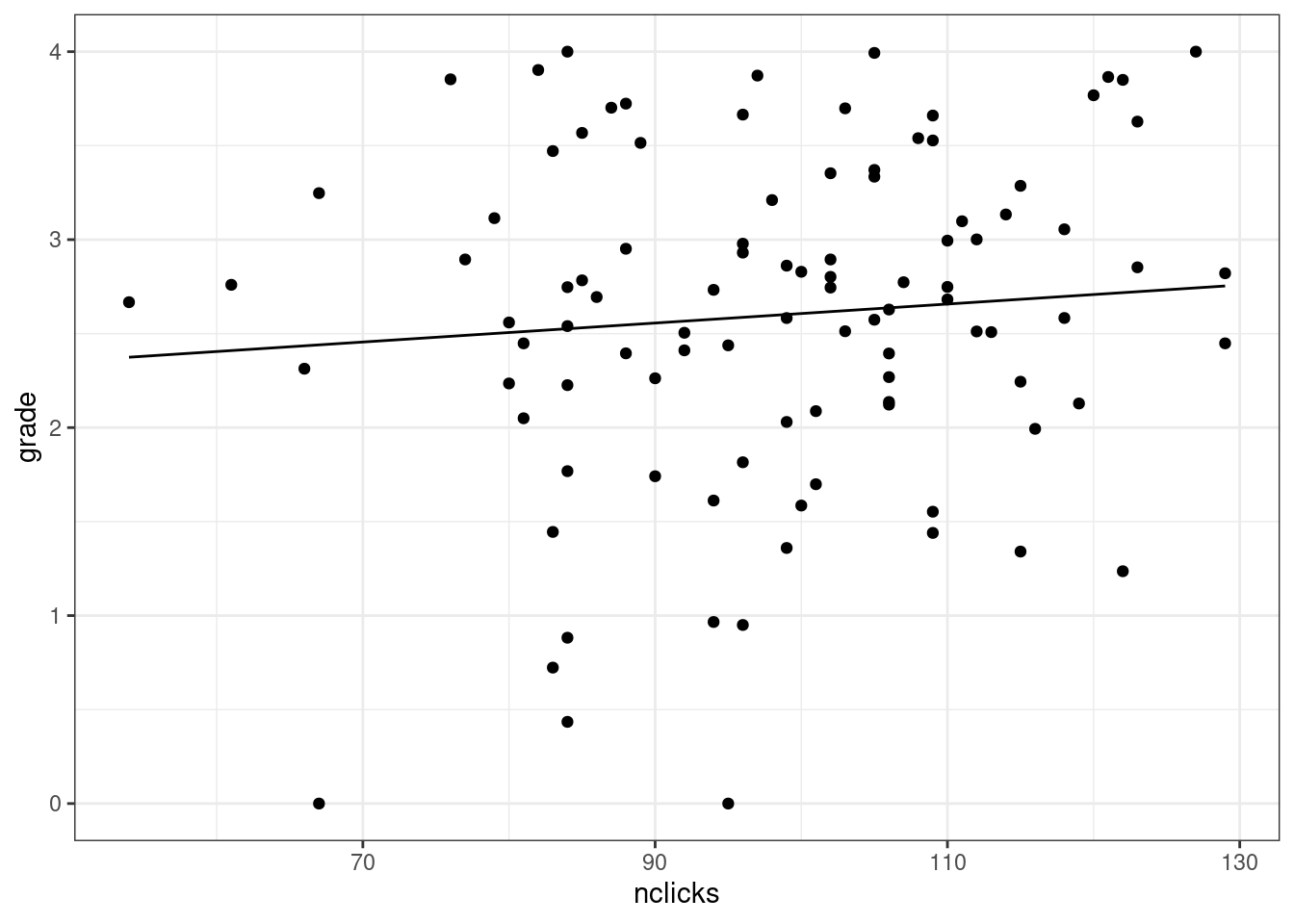
Figure 3.2: Partial effect plot of nclicks on grade.