For estimating structural equation models in R we will use the lavaan add-on package (Rosseel, 2012) for R. You can install it by typing install.packages("lavaan") in your R console window.
The main workhorse function for lavaan is called, simply, lavaan(). This is a powerful function that lets you specify a wide array of models. You can see all the options by looking at the help page (?lavaan::lavaan):
lavaan                 package:lavaan                  R Documentation

Fit a Latent Variable Model

Description:

     Fit a latent variable model.

Usage:

     lavaan(model = NULL, data = NULL, ordered = NULL,
            sampling.weights   = NULL,
            sample.cov = NULL, sample.mean = NULL, sample.th = NULL,
            sample.nobs = NULL,
            group = NULL, cluster = NULL, constraints = "",
            WLS.V = NULL, NACOV = NULL, ov.order = "model",
            slotOptions = NULL, slotParTable = NULL, slotSampleStats = NULL,
            slotData = NULL, slotModel = NULL, slotCache = NULL,
            sloth1 = NULL,
            ...)
The ... in the function syntax suggests there are more options than are listed, and the help page says “See lavOptions for a complete list.” And if you type lavOptions() you will see there are 113 additional options! This can be quite overwhelming for the novice user.
Fortunately, lavaan provides two ‘convenience’ functions that hide away some of this complexity and that automatically choose sensible defaults. These functions are:
function
description
sem()
Fit a structural equation model
cfa()
Fit a confirmatory factor analysis
In what follows, we’ll be using sem() to fit a path model. The function documentation indicates what options of lavaan are set to by default (see ?lavOptions for further information).
     The ‘sem’ function is a wrapper for the more general lavaan
     function, but setting the following default options: ‘int.ov.free
     = TRUE’, ‘int.lv.free = FALSE’, ‘auto.fix.first = TRUE’ (unless
     ‘std.lv = TRUE’), ‘auto.fix.single = TRUE’, ‘auto.var = TRUE’,
     ‘auto.cov.lv.x = TRUE’, ‘auto.efa = TRUE’, ‘auto.th = TRUE’,
     ‘auto.delta = TRUE’, and ‘auto.cov.y = TRUE’.
Many of these options are only relevant for models including latent variables, which our path models will not include. Thus, when using path analyses, these are the defaults you should keep in mind.
option setting
effect
int.ov.free=TRUE
intercepts of observed variables are not fixed to zero
auto.var=TRUE
residual variances for observed variables are set free
auto.cov.y=TRUE
covariances of endogenous variables are modeled and set free
7.2 Example: SEM vs regression
We will begin our practical introduction to path analysis with an example that represents a simple extension from ordinary regression modeling—namely, a situation where you have multiple response variables.
Let’s assume we’re interested in the social determinants of narcisissm and we have given a (subclinical) population a narcissism questionnaire (scale goes from 1-100).
To follow along, download the following files. NB: These files contain simulated (i.e., not real) data, so don’t draw any conclusions about narcissism from the analyses.
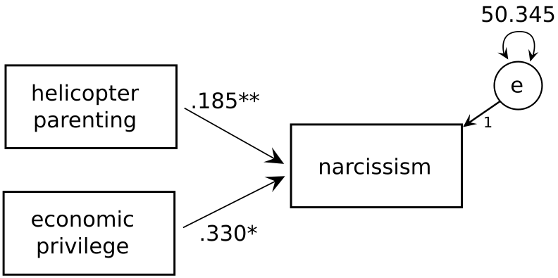
We might have the following theory of narcisissm, where parenting style (specifically, the degree of “helicopter” parenting where parents smother their child with attention) and economic privilege jointly determine the level of adult narcissism.
Here, the SEM framework wouldn’t buy us anything because we can fit this model using basic regression.
library("tidyverse") # for read_csvlibrary("lavaan") # for SEM; we'll need these functions later
This is lavaan 0.6-19
lavaan is FREE software! Please report any bugs.
narc_1 <-read_csv("data/narc_1.csv", col_types ="ddd")mod_reg <-lm(Narc ~ HP + EP, data = narc_1)summary(mod_reg)
Call:
lm(formula = Narc ~ HP + EP, data = narc_1)

Residuals:
     Min       1Q   Median       3Q      Max
-18.6504  -4.5028  -0.3351   4.4134  18.0993

Coefficients:
            Estimate Std. Error t value Pr(>|t|)
(Intercept) 42.62670    6.48476   6.573 4.31e-10 ***
HP           0.18531    0.06704   2.764  0.00625 **
EP           0.33032    0.12922   2.556  0.01133 *
---
Signif. codes:  0 '***' 0.001 '**' 0.01 '*' 0.05 '.' 0.1 ' ' 1

Residual standard error: 7.149 on 197 degrees of freedom
Multiple R-squared:  0.07027,   Adjusted R-squared:  0.06083
F-statistic: 7.445 on 2 and 197 DF,  p-value: 0.0007642
sem_formula <-'Narc ~ HP + EP'mod_sem <-sem(sem_formula, data = narc_1)summary(mod_sem, rsquare =TRUE)
lavaan 0.6-19 ended normally after 1 iteration

  Estimator                                         ML
  Optimization method                           NLMINB
  Number of model parameters                         3

  Number of observations                           200

Model Test User Model:

  Test statistic                                 0.000
  Degrees of freedom                                 0

Parameter Estimates:

  Standard errors                             Standard
  Information                                 Expected
  Information saturated (h1) model          Structured

Regressions:
                   Estimate  Std.Err  z-value  P(>|z|)
  Narc ~
    HP                0.185    0.067    2.785    0.005
    EP                0.330    0.128    2.576    0.010

Variances:
                   Estimate  Std.Err  z-value  P(>|z|)
   .Narc             50.345    5.034   10.000    0.000

R-Square:
                   Estimate
    Narc              0.070
You can see that the regression coefficients closely match the ones from the regression. We also get an estimate of the residual variance for the DV of 50.345, which is close to the “Residual standard error” in the regression model, because sqrt(50.345) = 7.095, which is close to 7.149.
The summary suggests that we have estimated 3 parameters. What are they? Let’s use lavaan’s parTable() function to see.
parTable(mod_sem)
  id  lhs op  rhs user block group free ustart exo label plabel  start    est
1  1 Narc  ~   HP    1     1     1    1     NA   0         .p1.  0.185  0.185
2  2 Narc  ~   EP    1     1     1    2     NA   0         .p2.  0.330  0.330
3  3 Narc ~~ Narc    0     1     1    3     NA   0         .p3. 50.345 50.345
4  4   HP ~~   HP    0     1     1    0     NA   1         .p4. 56.991 56.991
5  5   HP ~~   EP    0     1     1    0     NA   1         .p5.  1.423  1.423
6  6   EP ~~   EP    0     1     1    0     NA   1         .p6. 15.341 15.341
     se
1 0.067
2 0.128
3 5.034
4 0.000
5 0.000
6 0.000
The ‘free’ column counts the free parameters. You’ll note that Narc ~ HP, Narc ~ EP and Narc ~~ Narc are the (population) direct effects and variance that are being estimated. All the variances/covariances for the exogenous variables are just directly calculated from the sample, and so they have no standard errors (= 0).
We can also get confidence intervals using the parameterEstimates() function, which also puts the estimates in a table, making them easier to access for reporting.
parameterEstimates(mod_sem)
   lhs op  rhs    est    se      z pvalue ci.lower ci.upper
1 Narc  ~   HP  0.185 0.067  2.785  0.005    0.055    0.316
2 Narc  ~   EP  0.330 0.128  2.576  0.010    0.079    0.582
3 Narc ~~ Narc 50.345 5.034 10.000  0.000   40.477   60.212
4   HP ~~   HP 56.991 0.000     NA     NA   56.991   56.991
5   HP ~~   EP  1.423 0.000     NA     NA    1.423    1.423
6   EP ~~   EP 15.341 0.000     NA     NA   15.341   15.341
We can also get standardized estimates. The std.all column is the one you want to look at.
parameterEstimates(mod_sem, standardized =TRUE)
   lhs op  rhs    est    se      z pvalue ci.lower ci.upper std.lv std.all
1 Narc  ~   HP  0.185 0.067  2.785  0.005    0.055    0.316  0.185   0.190
2 Narc  ~   EP  0.330 0.128  2.576  0.010    0.079    0.582  0.330   0.176
3 Narc ~~ Narc 50.345 5.034 10.000  0.000   40.477   60.212 50.345   0.930
4   HP ~~   HP 56.991 0.000     NA     NA   56.991   56.991 56.991   1.000
5   HP ~~   EP  1.423 0.000     NA     NA    1.423    1.423  1.423   0.048
6   EP ~~   EP 15.341 0.000     NA     NA   15.341   15.341 15.341   1.000
  std.nox
1   0.025
2   0.045
3   0.930
4  56.991
5   1.423
6  15.341
7.2.2 Adding a second DV
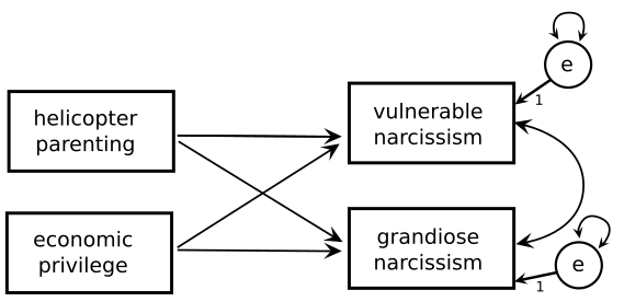
Up to this point using SEM doesn’t really buy us anything over and above ordinary regression. But the situation changes if we have more than one DV. Let’s say that instead of a single measure we had a measure of two types of narcissism: vulnerable narcissism (VN) and grandiose narcissism (GN), which, for the sake of example, let’s say are not mutually exclusive (i.e., a person can have a little bit of each).
We could perform two separate regressions, but this has the problem that each regression is performed independently of the other, which only makes sense if we are sure that the two DVs are totally uncorrelated. If they are correlated, then the estimates from this approach will be biased. Here, a SEM approach is useful because it can account for this covariance.
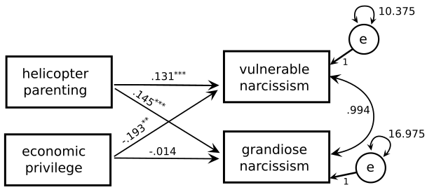
narc_2 <-read_csv("data/narc_2.csv",col_types ="dddd")sem_formula2 <-'VN ~ HP + EPGN ~ HP + EP'mod_sem2 <-sem(sem_formula2, data = narc_2)summary(mod_sem2, rsquare =TRUE)
lavaan 0.6-19 ended normally after 9 iterations

  Estimator                                         ML
  Optimization method                           NLMINB
  Number of model parameters                         7

  Number of observations                           200

Model Test User Model:

  Test statistic                                 0.000
  Degrees of freedom                                 0

Parameter Estimates:

  Standard errors                             Standard
  Information                                 Expected
  Information saturated (h1) model          Structured

Regressions:
                   Estimate  Std.Err  z-value  P(>|z|)
  VN ~
    HP                0.131    0.030    4.351    0.000
    EP               -0.193    0.058   -3.315    0.001
  GN ~
    HP                0.145    0.039    3.754    0.000
    EP               -0.014    0.074   -0.190    0.849

Covariances:
                   Estimate  Std.Err  z-value  P(>|z|)
 .VN ~~
   .GN                0.994    0.941    1.056    0.291

Variances:
                   Estimate  Std.Err  z-value  P(>|z|)
   .VN               10.375    1.037   10.000    0.000
   .GN               16.975    1.698   10.000    0.000

R-Square:
                   Estimate
    VN                0.125
    GN                0.066
Let’s have a look at the model estimates, including standardized coefficients, and add the (raw) coefficients to our path diagram.
parameterEstimates(mod_sem2, standardized =TRUE)
   lhs op rhs    est    se      z pvalue ci.lower ci.upper std.lv std.all
1   VN  ~  HP  0.131 0.030  4.351  0.000    0.072    0.191  0.131   0.288
2   VN  ~  EP -0.193 0.058 -3.315  0.001   -0.307   -0.079 -0.193  -0.219
3   GN  ~  HP  0.145 0.039  3.754  0.000    0.069    0.221  0.145   0.257
4   GN  ~  EP -0.014 0.074 -0.190  0.849   -0.160    0.132 -0.014  -0.013
5   VN ~~  VN 10.375 1.037 10.000  0.000    8.341   12.408 10.375   0.875
6   GN ~~  GN 16.975 1.698 10.000  0.000   13.648   20.302 16.975   0.934
7   VN ~~  GN  0.994 0.941  1.056  0.291   -0.850    2.838  0.994   0.075
8   HP ~~  HP 56.991 0.000     NA     NA   56.991   56.991 56.991   1.000
9   HP ~~  EP  1.423 0.000     NA     NA    1.423    1.423  1.423   0.048
10  EP ~~  EP 15.341 0.000     NA     NA   15.341   15.341 15.341   1.000
   std.nox
1    0.038
2   -0.056
3    0.034
4   -0.003
5    0.875
6    0.934
7    0.075
8   56.991
9    1.423
10  15.341
Rosseel, Y. (2012). Lavaan: An r package for structural equation modeling. Journal of Statistical Software, 48(2), 1–36. https://doi.org/10.18637/jss.v048.i02