Chapter 1 Importing data from different file formats into R

1.1 At a glance

File type	Extension	package::function
CSV	.csv	readr::read_csv()
Excel	.xls or .xlsx	readxl:read_excel()
Plain text	.txt	readr::read_lines()
SPSS	.sav	haven::read_sav()
Binary R data	.rds	readr::read_rds()
JSON	.json	jsonlite::fromJSON()

1.2 1. CSV

Most will be familiar with importing common-separated values (CSV) files using the read_csv() function offered in Tidyverse's 'readr' package. But what if your data is separated by tabs, semicolons, or other characters such as "|"? It is helpful to know that similar functions in 'readr' can readily help you import your data into R.

For tab-separated files (.tsv), use read_tsv().
For semicolon-separated files, where the comma is the decimal point not the separator, use read_csv2().

Here is the syntax.

#library(tidyverse)
tbl_csv <- read_csv("data/filename.csv")
tbl_csv2 <- read_csv2("data/filename.csv")
tbl_tsv <- read_tsv("data/filename.tsv")

1.2.1 Other delimiters

If your data are delimited by other characters such as "|", use read_delim() and specify the delimiter.

For example, if the text file looks like the dummy data below, we can see that "|" is the delimiter. (To try out the code below, you can copy the text, save it to a file and name it delim_data.txt.)

ParticipantID|Condition1|Condition2|Condition3|Control
130059284|0.4|0.01|0.2|0
290100722|0.3|0.02|0.3|1
387005398|0.5|0.01|0.4|0

dat_delim <- read_delim("data/delim_data.txt", delim = "|")

## Rows: 3 Columns: 5

## ── Column specification ─────────────────────────────────────────────────────────
## Delimiter: "|"
## dbl (5): ParticipantID, Condition1, Condition2, Condition3, Control

## 
## ℹ Use `spec()` to retrieve the full column specification for this data.
## ℹ Specify the column types or set `show_col_types = FALSE` to quiet this message.

R is now able to read the data as a tibble:

ParticipantID	Condition1	Condition2	Condition3	Control
130059284	0.4	0.01	0.2	0
290100722	0.3	0.02	0.3	1
387005398	0.5	0.01	0.4	0

1.2.2 Changing the data type for each column

Sometimes we want to specify the data type for each column. When we load the data, R generates a message (as above) to indicate the data type of each column. In our case, R has recognised all 5 columns as doubles or dbl, which is a class of numeric data, similar to float in other programming languages.

Let's say we want ParticipantID as characters and Control as boolean (i.e., TRUE or FALSE, known as logical in R), we can add the col_types argument.

In the code below, col_types = "c???l" specifies that for our 5 columns, we want to change the data type of ParticipantID to character and Control to logical. Since we don't need to change the data type for Condition1, Condition2, and Condition3, we use ? to allow R to guess.

dat_delim_col_types <- read_delim("data/delim_data.txt", delim = "|", col_types = "c???l")  
spec(dat_delim_col_types) # check column data types

## cols(
##   ParticipantID = col_character(),
##   Condition1 = col_double(),
##   Condition2 = col_double(),
##   Condition3 = col_double(),
##   Control = col_logical()
## )

You can specify the data type you want by using one character to represent each column. The column types are: c = character, i = integer, n = number, d = double, l = logical, f = factor, D = date, T = date time, t = time, ? = guess, or _/- to skip the column.

The argument col_types is also used in other functions in this tutorial, including read_excel() for Excel data and read_table() for reading text as a tibble.

1.2.3 Write data to CSV

After loading data from various file formats and having cleaned and wrangled the data, you may want to save the tibble to .csv. This would allow you to view the data later or share the file with others without having to run the whole R script again.

Here is the syntax.

write_csv(cleaned_data, "cleaned_data.csv")

Read more about 'readr' package and see the cheat sheet here. Related packages include 'readxl' (detailed below) and 'googlesheets4' which allows you to read data from and write data to Google Sheets.

1.3 2. Excel (.xls or .xlsx)

We use the 'readxl' package, part of Tidyverse, to read Excel data into R. Try out the 'readxl' functions below either using your data or download the Demo.xlsx file here (111KB). The data have been adapted from a public domain dataset, Chocolate Bar Ratings (Tatman, 2017), which contains expert ratings of 1700 chocolate bars.

For demonstration purposes, the demo file contains 3 sheets, sorted by chocolate makers' company names starting A to G (Sheet 1), H to Q (Sheet 2), and R to Z (Sheet 3). You can access sheets either by name or by index.

# Suggested: install 'readxl' and load separately
library(readxl) 
dat_excel<- readxl::read_excel("data/Demo.xlsx") # by default, this loads Sheet 1 only.

Company (Maker-if known)	Specific Bean Origin or Bar Name	REF	Review Date	Cocoa Percent	Company Location	Rating	Bean Type	Broad Bean Origin
A. Morin	Agua Grande	1876	2016	0.63	France	3.75	¬†	Sao Tome
A. Morin	Kpime	1676	2015	0.70	France	2.75	¬†	Togo
A. Morin	Atsane	1676	2015	0.70	France	3.00	¬†	Togo
A. Morin	Akata	1680	2015	0.70	France	3.50	¬†	Togo
A. Morin	Quilla	1704	2015	0.70	France	3.50	¬†	Peru
A. Morin	Carenero	1315	2014	0.70	France	2.75	Criollo	Venezuela

If you check dat_excel (using either summary() from base R or dplyr::glimpse()), you will see that if you don't specify the sheet, only the first sheet is loaded.

Use the 'readr' function excel_sheets() to get a list of sheet names.

excel_sheets("data/Demo.xlsx")

## [1] "Companies_A_to_G" "Companies_H_to_Q" "Companies_R_to_Z"

Then, you can specify which sheet you want to load, by sheet name or index.

sheet_by_name <- read_excel("data/Demo.xlsx", sheet = "Companies_H_to_Q") #load sheet 2 by name
sheet_by_index <- read_excel("data/Demo.xlsx", sheet = 3) #load sheet by index

1.3.1 Dealing with formulas and formatted cells

Sometimes you may encounter Excel data that contain formulas written in VBA macros or highlighted cells in yellow or in bold.

If you want to extract the formulas or formatted cells from Excel, there are R functions that could help. The 'tidyxl' package has the function tidyxl::xlsx_cells() which reads the property of each cell in an Excel spreadsheet, such as the data type, formatting, whether it is a formula, the cell's font, height and width. Please refer to the 'tidyxl' vignette.

However, proceed with caution! Spreadsheet errors, either due to human mistakes or Excel's autocorrect functions, have raised reproducibility concerns in behavioural science and genetics research (see Alexander, 2013; Lewis, 2021). If you see strange behaviour from your Excel data, check the file: Are the formulas referring to the correct cells? Has a large number been autocorrected into a date? When in doubt, open the file in Excel to check.

1.4 3. Plain text (.txt)

When your data are in .txt files, you can either use readLines() from base or readr::read_lines() from Tidyverse. Here, we use the latter, as it runs faster for large datasets.

As an example, we use a simple dataset from Stigliani and Grill-Spector (2018), a neuroscience study. You can click here to download the data directly (392 bytes).

First, we read in the file to see what it contains.

#load the tidyverse package
readr_text <- read_lines(("data/Exp1_Run1.txt"), n_max=10)
readr_text

##  [1] "Exp1 conditions: 2s, 4s, 8s, 15s, 30s"
##  [2] "Run duration (s): 276"                
##  [3] ""                                     
##  [4] "Trial Condition Onset Duration Image" 
##  [5] "1 8s 12 8 scrambled-260.jpg"          
##  [6] "2 2s 32 2 scrambled-191.jpg"          
##  [7] "3 4s 46 4 scrambled-481.jpg"          
##  [8] "4 30s 75 30 scrambled-996.jpg"        
##  [9] "5 15s 117 15 scrambled-355.jpg"       
## [10] "6 8s 144 8 scrambled-47.jpg"

The n_max argument above specifies how many lines of data you would like to read. We can see that we need to skip the first 3 lines for the data to form a tibble. We use read_table() to create the tibble.

dat_txt <- read_table(file = "data/Exp1_Run1.txt", skip = 3) # skip first 3 lines

Trial	Condition	Onset	Duration	Image
1	8s	12	8	scrambled-260.jpg
2	2s	32	2	scrambled-191.jpg
3	4s	46	4	scrambled-481.jpg
4	30s	75	30	scrambled-996.jpg
5	15s	117	15	scrambled-355.jpg
6	8s	144	8	scrambled-47.jpg
7	15s	177	15	scrambled-520.jpg
8	2s	204	2	scrambled-512.jpg
9	4s	218	4	scrambled-262.jpg
10	30s	234	30	scrambled-201.jpg

By default, the argument col_names is set to TRUE, so that the first row of text input will be imported as column names. If you set it to FALSE, the column names will be generated automatically as X1, X2, X3, etc.

If you want to rename columns in the same line of code, you can enter a character vector for col_names. For example:

dat_txt_new_column_names <- read_table(file = "data/Exp1_Run1.txt", skip = 4, col_names = c("Trial_new", "Condition_new", "Onset_new", "Duration_new", "Image_new"))
#since we are renaming the columns, we skip 4 lines

The column names will become:

Trial_new	Condition_new	Onset_new	Duration_new	Image_new
1	8s	12	8	scrambled-260.jpg

Of course, another way to rename columns would be using dplyr::rename(data, new_name = old_column_name) or dplyr::rename_with(data, function). For example, running the following will turn all column names to upper case. Try it yourself and see.

dat_txt_upper <- rename_with(dat_txt, toupper)

1.5 4. SPSS data (.sav)

We will use the 'haven' package, which is part of Tidyverse, to import SPSS data into a tibble.

The example below uses SPSS data from Norman et al.(2021), Study 2, which examines adult identity. You can click here to download the data directly (564KB).

# Suggested: install the package 'haven' and load it in addition to Tidyverse. 
library(haven)
dat_sav <- haven::read_sav("data/EA Across Age Data.sav")

The tibble dat_sav has 173 columns and 658 rows. If you only need to load a subset of columns, the col_select argument allows you to select columns by index or by column name. Below is an example of using col_select and what the output looks like. This would be an alternative to dplyr::select().

#load the first 8 columns
dat_select_by_index <- read_sav("data/EA Across Age Data.sav", col_select=(1:8))

StartDate	EndDate	Progress	Duration_in_seconds	IC	IDEA_1_1	IDEA_1_2	IDEA_1_3
2019-10-02 18:00:53	2019-10-02 18:12:17	100	684	1	3	4	2
2019-10-12 13:18:40	2019-10-12 13:30:16	100	696	1	3	4	3
2019-10-12 15:03:10	2019-10-12 15:12:03	100	533	1	3	4	3
2019-10-12 15:02:12	2019-10-12 15:12:55	100	642	1	3	4	4
2019-10-12 15:22:10	2019-10-12 15:37:06	100	895	1	4	4	4
2019-10-12 15:43:36	2019-10-12 15:53:44	100	608	1	4	3	4

#load columns with name starting with "IDEA"
dat_select_by_colname <- read_sav("data/EA Across Age Data.sav", 
                                  col_select = starts_with("IDEA"))

IDEA_1_1	IDEA_1_2	IDEA_1_3	IDEA_1_4	IDEA_1_5	IDEA_1_6	IDEA_1_7	IDEA_1_8	IDEA_1_9	IDEA_1_10	IDEA_1_11	IDEA_1_12	IDEA_1_13	IDEA_1_14	IDEA_1_15	IDEA_2_1	IDEA_2_2	IDEA_2_3	IDEA_2_4	IDEA_2_5	IDEA_2_6	IDEA_2_7	IDEA_2_8	IDEA_2_9	IDEA_2_10	IDEA_2_11	IDEA_2_12	IDEA_2_13	IDEA_2_14	IDEA_2_15	IDEA_2_16	IDEA_Total
3	4	2	4	3	3	4	4	4	3	4	4	2	2	3	3	3	3	4	4	4	4	4	4	4	3	4	4	4	3	2	3.419355
3	4	3	3	3	3	4	4	3	3	4	3	2	3	3	3	4	3	3	3	3	3	4	3	4	4	4	4	3	2	2	3.225807
3	4	3	3	4	3	4	4	4	3	4	4	2	3	4	4	4	3	3	4	4	4	4	4	3	3	4	4	4	4	4	3.612903
3	4	4	4	3	2	4	4	4	2	4	4	1	3	4	3	4	3	4	4	3	3	3	3	2	4	4	4	4	4	4	3.419355
4	4	4	4	3	3	4	4	4	4	4	4	3	3	4	4	4	3	4	3	4	4	3	3	4	4	4	4	4	4	4	3.741935
4	3	4	3	3	3	4	4	4	3	4	4	1	2	3	3	4	2	2	3	4	3	4	2	3	2	4	4	4	2	3	3.161290

1.6 5. Binary R data (.rds)

RDS files store datasets in a compressed format to save storage space. Additionally, RDS preserves data types such as dates and factors, so we don't need to worry about redefining data types after reading the file into R.

To read .rds files, use either readRDS() from baseR or read_rds() from Tidyverse's 'readr' package. We use Tidyverse in the example below.

The example below uses data from Lukavsky (2018), Experiment 1. The study investigates participants' ability to recognise what they have seen in their central and peripheral vision. You can click here to download the data directly (185KB).

#library(tidyverse)
dat_binary <- read_rds("data/exp1.rds")

You will see that this dataset has over 5300 rows and 26 columns. Here is what the first 6 lines look like.

id	version	block	trial	image	response	rt	fix_ok	new_sample	d	mx	my	sofa	focus	code_in	code_out	category_in	category_out	image_in	image_out	code_target	category_target	image_target	conflicting	correct
1	1	3	1	NB29_MS02.jpg	1	0.778776	1	1	11.08871	8.599976	-7.000000	0.200060	in	N	M	NB	MS	NB29	MS02	N	NB	NB29	TRUE	TRUE
1	1	3	2	NF26_NF03.jpg	1	0.271486	1	1	14.81656	11.200012	9.700012	0.199956	in	N	N	NF	NF	NF26	NF03	N	NF	NF26	FALSE	TRUE
1	1	3	3	NM16_NB13.jpg	1	0.315025	1	1	21.95861	-19.700012	-9.700012	0.200115	in	N	N	NM	NB	NM16	NB13	N	NM	NM16	FALSE	TRUE
1	1	3	4	MP09_NR18.jpg	-1	0.354698	1	1	19.93792	4.599976	19.400024	0.200100	in	M	N	MP	NR	MP09	NR18	M	MP	MP09	TRUE	TRUE
1	1	3	5	MH13_NB16.jpg	-1	0.218628	1	1	14.11525	5.000000	13.200012	0.200121	in	M	N	MH	NB	MH13	NB16	M	MH	MH13	TRUE	TRUE
1	1	3	6	MM18_NM10.jpg	-1	0.514552	1	1	37.04375	-31.799988	-19.000000	0.200095	in	M	N	MM	NM	MM18	NM10	M	MM	MM18	TRUE	TRUE

1.7 6. JSON

JSON files store nested lists or data in a tree-like structure. We will use the 'jsonlite' package to view and access the data in R.

You can download an example.json file here (4KB). The data are sourced from the International Union for Conservation of Nature Red List of Threatened Species.

# install the 'jsonlite' package first
library(jsonlite)
dat_json <- fromJSON(txt="data/example.json", simplifyDataFrame = FALSE)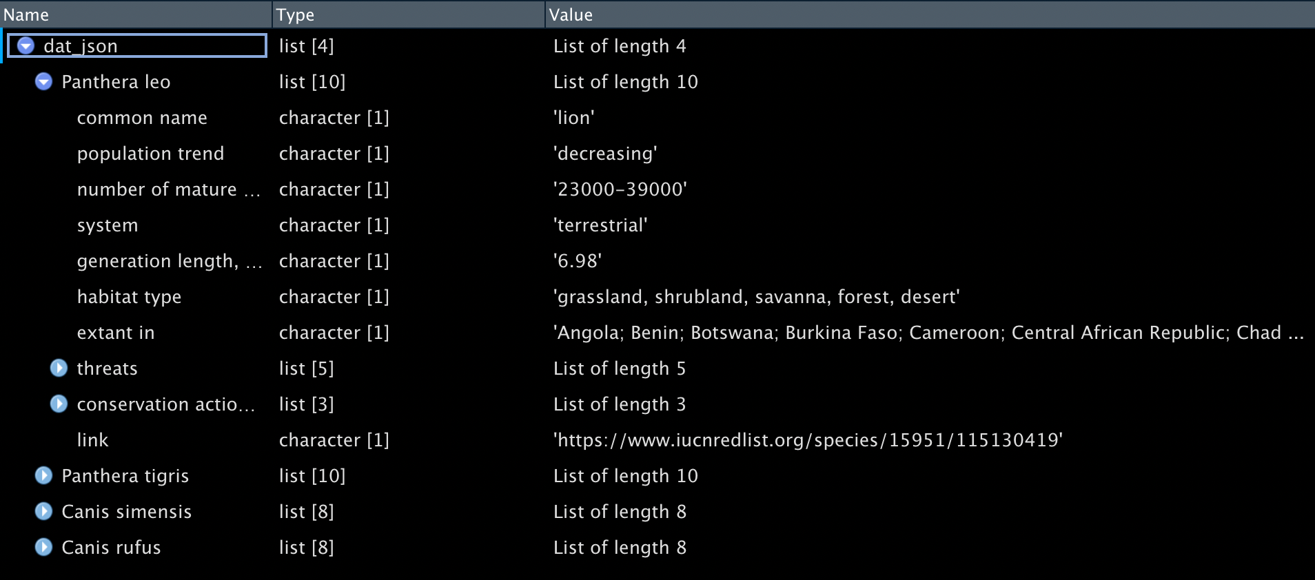

From the RStudio Viewer you would see that the data contain information about 4 animals.

You can also navigate the data using names() from base or simply type dat_json$"Panthera leo". The dollar sign $ refers to a variable or column. In RStudio, as you type in data_object_name$, the available variables or columns will be shown for your choice.

names(dat_json) #gets names of what's in the object
names(dat_json$`Panthera tigris`) # get variable names one level down. Use `` or "" for variable names containing spaces.

## [1] "Panthera leo"    "Panthera tigris" "Canis simensis"  "Canis rufus"    
##  [1] "common name"                   "population trend"             
##  [3] "number of mature individuals"  "system"                       
##  [5] "generation length, in years"   "habitat type"                 
##  [7] "Extant in"                     "threats"                      
##  [9] "conservation actions in place" "link"

Use as_tibble() to put the data into a tibble for further processing.

tiger_conservation <- dat_json$`Panthera tigris`$`conservation actions in place` %>% as_tibble()

in-place land/water protection	in-place species management	in-place education
occurs in at least one protected area	harvest management plan; successfully reintroduced or introduced benignly; subject to ex-situ conservation	subject to recent education and awareness programmes; included in international legislation; subject to any international management / trade controls

You can transpose the tibble so it is easier to read.

tiger_conversation_long_view <- tiger_conservation %>% pivot_longer(cols = everything())

name	value
in-place land/water protection	occurs in at least one protected area
in-place species management	harvest management plan; successfully reintroduced or introduced benignly; subject to ex-situ conservation
in-place education	subject to recent education and awareness programmes; included in international legislation; subject to any international management / trade controls

1.8 Reference

Alexander, R. (2013, April 20). Reinhart, Rogoff... and Herndon: The student who caught out the profs. BBC. https://www.bbc.com/news/magazine-22223190

International Union for Conservation of Nature. (n.d.). The IUCN Red List of Threatened Species. https://www.iucnredlist.org

Lewis, D. (2021, August 25). Autocorrect errors in Excel still creating genomics headache. Nature. https://www.nature.com/articles/d41586-021-02211-4

Lukavsky, J. (2018, December 5). Scene categorization in the presence of a distractor. Retrieved from osf.io/849wm

Norman, K., Hernandez, L., & Obeid, R. (2021, January 12). Study 2. Who Am I? Gender Differences in Identity Exploration During the Transition into Adulthood. Retrieved from osf.io/agfvz

Stigliani, A., & Grill-Spector, K. (2018, July 5). Temporal Channels. https://doi.org/10.17605/OSF.IO/MW5PK

Tatman, R. (2017). Chocolate Bar Ratings. Kaggle Datasets. https://www.kaggle.com/rtatman/chocolate-bar-ratings

1 Importing data from different file formats into R