2A Lab 4 Week 5

This is the pair coding activity related to 4  Data viz I.

Task 1: Open the R project for the lab

Task 2: Create a new .Rmd file

… and name it something useful. If you need help, have a look at 1.3 Activity 2: Create a new R Markdown file.

Task 3: Load in the library and read in the data

The data should already be in your project folder. If you want a fresh copy, you can download the data again here: data_pair_coding.

We are using the package tidyverse today, and the datafile we should read in is dog_data_clean_wide.csv.

Task 4: Create an appropriate plot

Pick any single or two categorical variables from the Binfet dataset and choose one of the appropriate plot choices. Things to think about:

• Select your categorical variable(s): GroupAssignment, Year_of_Study, Live_Pets, and/or Consumer_BARK
• Decide on the plot you want to display: barchart, stacked barchart, percent stacked barchart, or grouped barchart
• You may need to convert your variables into factors
• Think about what you want to do with missing data
• Pick a colour scheme (manual or pre-defined colour palette)
• Tidy the axes labels
• Decide whether you need a legend or not, and if so, where you would want to place it
• Remove the gap between the bottom of the chart and the bars
• Pick a theme

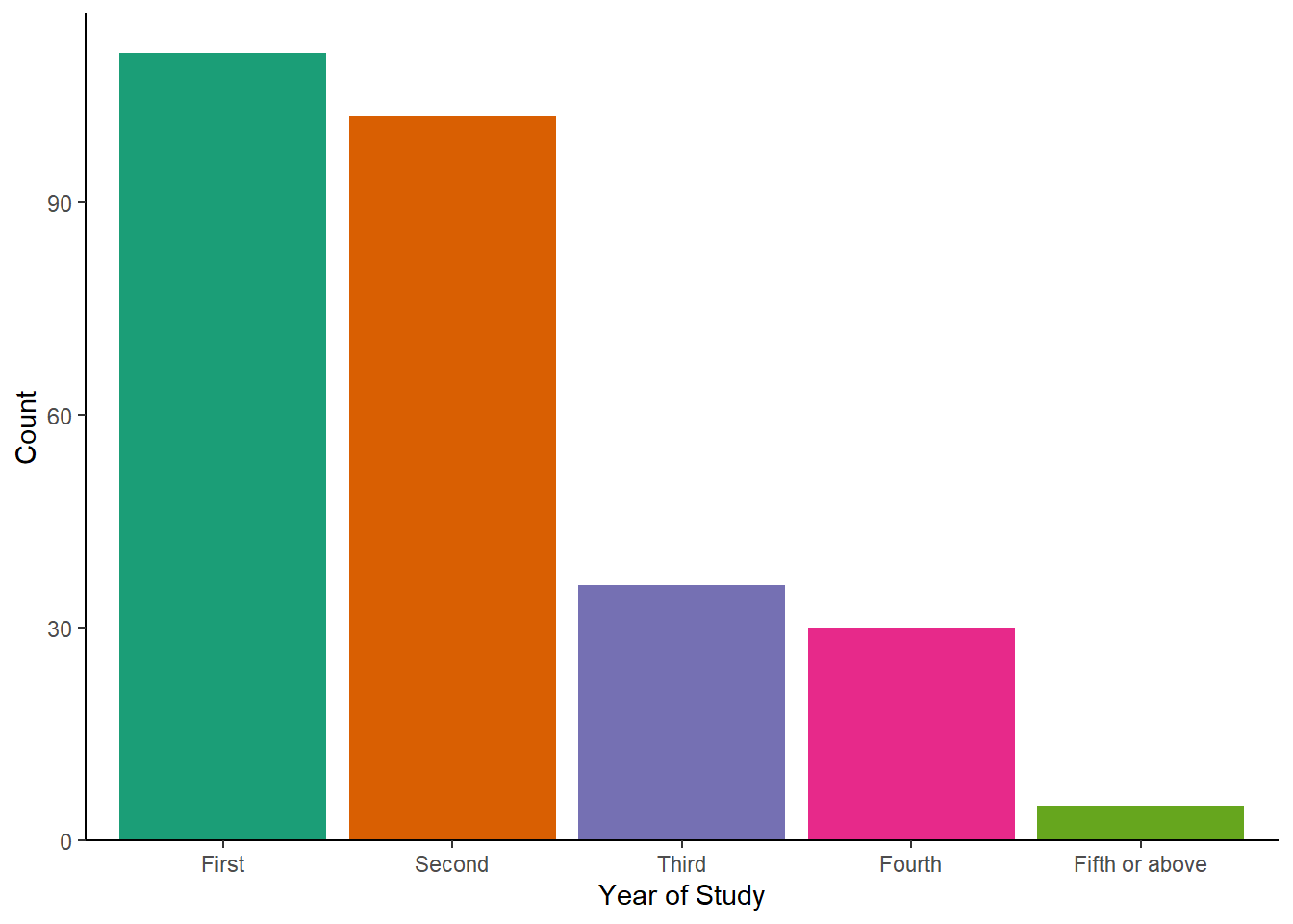
Possible solution for a plot with 1 categorical variable

Converting some variables into factors

dog_data_wide <- dog_data_wide %>% 
  mutate(Year_of_Study = factor(Year_of_Study,
                                levels = c("First", "Second", "Third", "Fourth", "Fifth or above")))

Now we can plot

ggplot(dog_data_wide, aes(x = Year_of_Study, fill = Year_of_Study)) +
  geom_bar() + 
  scale_fill_brewer(
    palette = "Dark2",
    guide = "none") + 
  scale_x_discrete(name = "Year of Study") + 
  scale_y_continuous(name = "Count",
                     expand = expansion(mult = c(0, 0.05))) + 
  theme_classic()

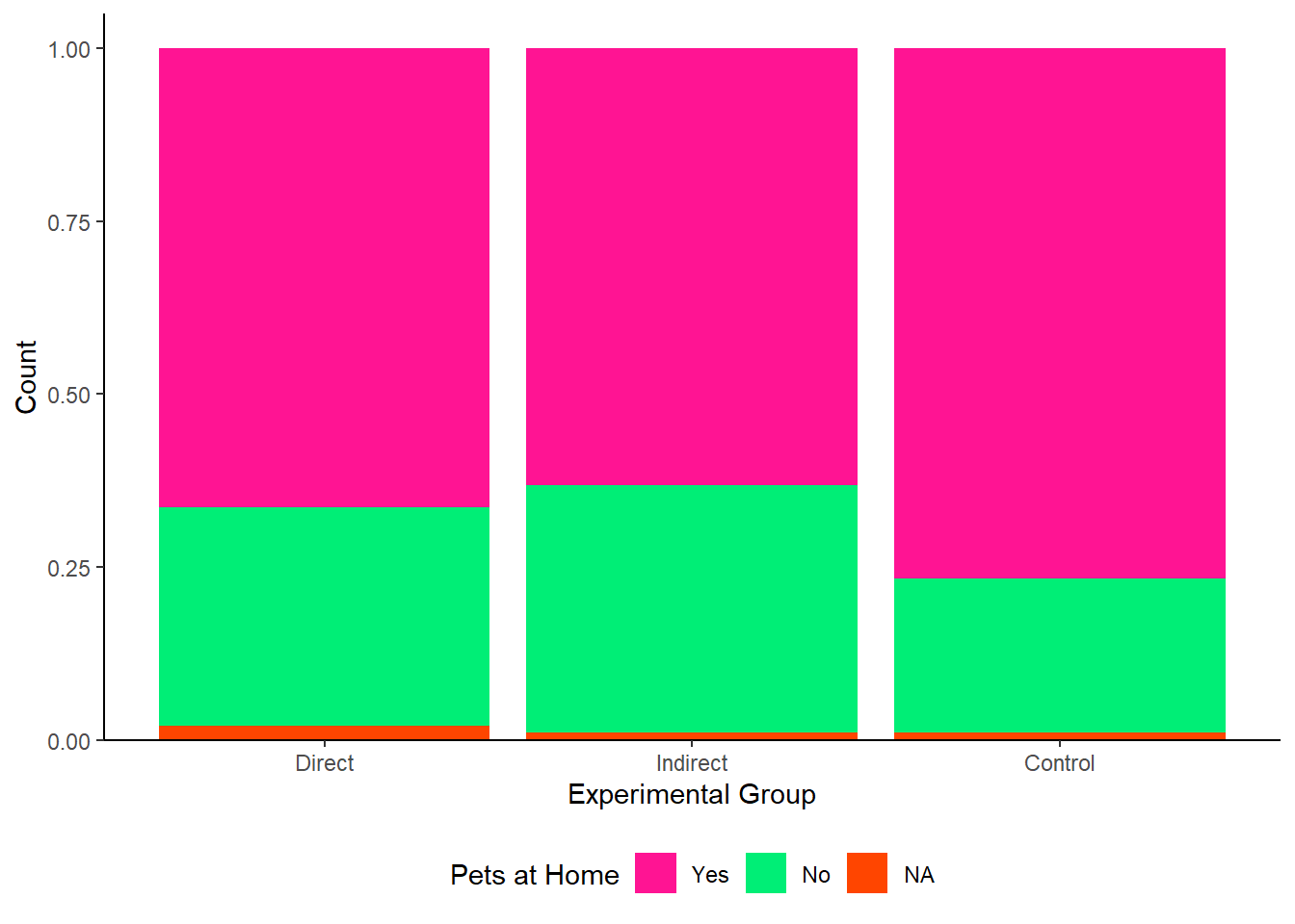
Possible solution for a plot with 2 categorical variables

Converting some variables into factors

dog_data_wide <- dog_data_wide %>% 
  mutate(GroupAssignment = factor(GroupAssignment,
                                  levels = c("Direct", "Indirect", "Control")))

Now we can plot

ggplot(dog_data_wide, aes(x = GroupAssignment , fill = Live_Pets)) +
  geom_bar(position = "fill") + 
  labs(x = "Experimental Group", y = "Count", fill = "Pets at Home") +
  scale_fill_manual(values = c('deeppink', 'springgreen2'), na.value = 'orangered',
                    labels = c("Yes", "No")) +
  scale_y_continuous(expand = expansion(mult = c(0, 0.05))) +
  theme_classic() + 
  theme(legend.position = "bottom")