
2B Lab 7 Week 9
This is the pair coding activity related to Chapter 13.
Task 1: Open the R project for the lab
Task 2: Create a new .Rmd file
Task 3: Load in the library and read in the data
The data should already be in your project folder. If you want a fresh copy, you can download the data again here: data_pair_coding.
We are using the packages afex, tidyverse, and performance today, and need to read in dog_data_clean_long.
Task 4: Tidy data & Selecting variables of interest
Let’s define a potential research question:
How does the Year of Study (1st, 2nd, 3rd, 4th, 5th or above) and Time point (pre- and post-intervention scores) affect perceived Happiness?
This is a 2 x 5 mixed factorial ANOVA, with one (Stage: pre vs. post) and one (year of study: 1st, 2nd, 3rd, 4th, 5th or above). The variable is self-reported Happiness Score.
Not much tidying to do today. All the variables and average scores are already tidied up in dog_data_long. We just need to check for missing values in our variables of interest. Best to do this on a reduced dataframe.
- select the variables of interest and store them in a new data object called
dog_factorial_anova - check for missing values and remove participants who did not have pre- and post-intervention Happiness recorded
Task 5: Model creating & Assumption checks
Now, let’s create our ANOVA model.
According to our research question we have the following model variables (use the spelling of the variable names in dog_factorial_anova):
- Dependent Variable (DV): , assessed pre- and post-intervention
- Independent Variable 1 (IV 1): (1st, 2nd, 3rd, 4th, 5th or above)
- Independent Variable 2 (IV 2): (pre- and post-intervention scores)
As a reminder, the ANOVA model has the following structure:
Let’s use this template to fill in our variables of interest and store the model in a separate object called mod. The effect size should be partial eta squared ("pes"):
Let’s check some assumptions.
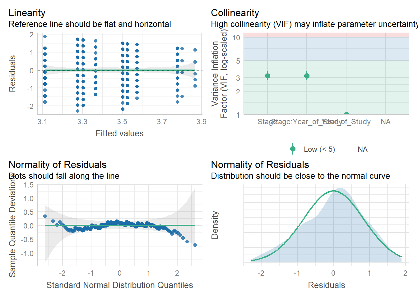
OK: There is not clear evidence for different variances across groups (Levene's Test, p = 0.882).Are the following assumptions met or violated?
- Assumption 1: Continuous DV?
- Assumption 2: Data are independent?
- Assumption 3: Normality?
- Assumption 4: Homoscedasticity?
Task 6: Interpreting the output
Call the model object to view the ANOVA results:
Anova Table (Type 3 tests)

Response: SHS
               Effect     df  MSE         F  pes p.value
1       Year_of_Study 4, 278 1.34      1.58 .022    .179
2               Stage 1, 278 0.09 19.86 *** .067   <.001
3 Year_of_Study:Stage 4, 278 0.09      0.45 .006    .772
---
Signif. codes:  0 '***' 0.001 '**' 0.01 '*' 0.05 '+' 0.1 ' ' 1
How do you interpret the results?