2B Lab 2 Week 3

This is the pair coding activity related to 9  Correlations.

Task 1: Open the R project for the lab

Task 2: Create a new .Rmd file

… and name it something useful. If you need help, have a look at 1.3 Activity 2: Create a new R Markdown file.

Task 3: Load in the library and read in the data

The data should already be in your project folder. If you want a fresh copy, you can download the data again here: data_pair_coding.

We are using the packages tidyverse and correlation today. If you have already worked through this chapter, you will have all the packages installed. If you have yet to complete 9  Correlations, you will need to install the package correlation (see 1.5.1 Installing packages for guidance if needed).

We also need to read in dog_data_clean_wide.csv. Again, I’ve named my data object dog_data_wide to shorten the name but feel free to use whatever object name sounds intuitive to you.

Task 4: Tidy data & Selecting variables of interest

Step 1: Select the variables of interest. We need 2 continuous variables today, so any of the pre- vs post-test comparison will do. I would suggest happiness ratings (i.e., SHS_pre, SHS_post). Also keep the participant id RID. Store them in a new data object called dog_happy.

Step 2: Check for missing values and remove participants with missing in either pre- or post-ratings.

Step 3: Convert participant ID into a factor

Solution for Tasks 3 and 4

## Task 3
library(tidyverse)
library(correlation)

dog_data_wide <- read_csv("dog_data_clean_wide.csv")


## Task 4
dog_happy <- dog_data_wide %>%
  # Step 1
  select(RID, SHS_pre, SHS_post) %>% 
  # Step 2
  drop_na() %>% 
  # Step 3
  mutate(RID = factor(RID))

Task 5: Re-create the scatterplot below

`geom_smooth()` using formula = 'y ~ x'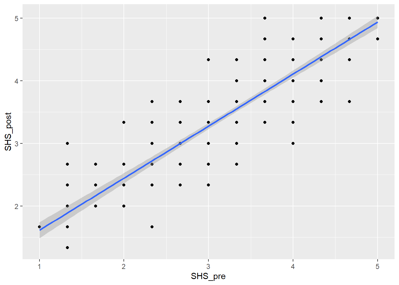

Solution

ggplot(dog_happy, aes(x = SHS_pre, y = SHS_post)) +
  geom_point() +
  geom_smooth(method = "lm")

Task 6: Assumptions check

We can either do the assumption check by looking at the scatterplot above or we can run the code plot(lm(SHS_pre~SHS_post, data = dog_happy)) and assess the assumptions there. Either way, it should give you similar responses.

• Linearity: a non-linearlinear relationship
• Normality: residuals are approximately normally distributednot normally distributed
• Homoscedasticity: There is
  heteroscedasticity as the residuals show a distinct pattern homoscedasticity as there is no distinct pattern in the residuals
• Outliers: the data has some outliersthe data does not have any clear outliers

What is your conclusion from the assumptions check?

All assumptions hold. Therefore, we are conducting a parametric test, specifically Pearson’s correlation. Some assumptions are violated. Therefore, we are conducting a non-parametric test, specifically Spearman’s correlation. All assumptions are violated. Therefore, we are conducting a non-parametric test, specifically Spearman’s correlation.

Task 7: Compute a Pearson correlation & interpret the output

• Step 1: Compute the Pearson correlation. The structure of the function is as follows:

correlation(data = your_dataframe,
            select = "variable1",
            select2 = "variable2",
            method = "Pearson",
            alternative = "two.sided")

The default method argument is Pearson, but if you thought any of the assumptions were violated and conduct a Spearman correlation instead, change the method argument to”Spearman”.

Solution

correlation(data = dog_happy,
            select = "SHS_pre",
            select2 = "SHS_post",
            method = "Pearson",
            alternative = "two.sided")

Parameter1	Parameter2	r	CI	CI_low	CI_high	t	df_error	p	Method	n_Obs
SHS_pre	SHS_post	0.8842169	0.95	0.855856	0.9072765	31.73394	281	0	Pearson correlation	283

# alternative because there are only 2 numeric columns in `dog_happy`
correlation(dog_happy)

• Step 2: Interpret the output

A Pearson correlation revealed a strongmoderately strongweak, positivenegative, and statistically significantnon-significant relationship between happiness before and after the dog intervention, r() = , p , 95% CI = [, ]. We therefore fail to reject the null hypothesisreject the null hypothesis in favour of H1.

Important

In the write-up paragraph above, the open fields accepted answers with 2 or 3 decimal places as correct. However, in your reports, ensure that correlation values are reported with 3 decimal places.