5 Allen et al. (2021): Promoting statistic selection skills
In this data analysis journey, we focus on inferential statistics after some data wrangling to apply the whole pipeline of skills that you are developing. We expect you can apply basic data wrangling tasks like creating and modifying variables, calculate descriptive statistics, create plots such as bar plots and boxplots, and apply simple linear regression techniques. We will also include some bonus sections at the end to flag where you could apply alternative modelling techniques depending where you are in your learning journey.
Assumed level: Analysing one outcome/DV and one predictor/IV, such as semester 1 in Undergraduate Level 2 or Postgraduate RM1. For the bonus analyses, handling multiple predictors/IVs, such as semester 2 in Undergraduate Level 2 or Postgraduate RM2.
5.1 Task preparation
5.1.1 Introduction to the data set
For this task, we are using open data from Allen et al. (2021) who were interested in improving students’ statistic selection skills. The abstract of their article is:
Psychology students struggle to recall, recognize, or explain how they would select appropriate statistics for common research designs. These selection skills are underpinned by structural awareness, which is the ability to look past the surface (or topic) features of a research design and focus instead on its deep structural characteristics. Although most psychology undergraduates display limited structural awareness, it can be trained. In this preregistered experiment, we designed and evaluated a novel method of training structural awareness. This training method made use of StatHand, a free iOS and web application, in scaffolded activities designed to highlight how the structural (but not surface) characteristics of a research design determine the selection of an appropriate statistical analysis. Bayesian analyses clearly indicated that this training was effective. Specifically, trained undergraduate psychology students (n 50) outperformed an untrained control group (n 52) on 5 measures of structural awareness (performance on 2 sets of triad judgment tasks, 2 sets of explanation tasks, and a scenario generation task) immediately following training, and again 1 week later (\(\delta\) = 0.71 to 1.60). At both time points, the trained students also showed greater selection skills than the untrained control students (\(\delta\) = 0.52 and 0.57). Finally, on 5 of these 6 outcome measures, the trained students showed no decrease in performance between the 2 time points. Educators are encouraged to consider how they can adapt our methods and materials for deployment in a classroom context or online activities.
In summary, they were interested in how you can train psychology students to improve their skills in identifying a statistical test. They wanted to develop “structural awareness” - the ability to identify structural characteristics of a data set and see past surface details.
Before we move on, read the abstract closely and try to identify the elements of the design (testing your own structural awareness, if you will…) to guide how we will need to wrangle the data and identify an appropriate statistical test. Once you have answered the questions, check your understanding against the answers below.
The first independent variable in the study is .
The first independent variable has levels. The two levels are . We can describe the first independent variable as .
The second independent variable in the study is .
The second independent variable has levels. The two levels are . We can describe the first independent variable as .
There are main dependent variables to measure structural awareness and selection skills.
There are two main independent variables in the study. The first is training as a between-subjects IV, where participants were randomly allocated to one of two groups:
Statistical selection training using StatHand (Training).
A control task with an unrelated iPad app (Control).
The second IV was within-subjects for measuring the outcomes over two time points:
Time 1 was the initial training phase.
Time 2 was usually 7 days after the training phase.
There were six different dependent variables in the study. Five measured structural awareness using things like a triad judgement task, and a sixth measured selection skills for suggesting an appropriate statistical test to a range of scenarios.
The authors posed three hypotheses which we will test after some data wrangling:
“We hypothesized that, compared to untrained students, trained students would perform better on five tasks reflecting structural awareness”. For the purposes of this chapter, we will just focus on one outcome relating to structural awareness: Surface-Deep (S-D) Triad.
“We hypothesized that, compared to untrained students, trained students would demonstrate stronger statistic selection skills.”
“We hypothesized that these effects would be evident immediately following training (or a control task) and again following a 1-week delay”.
5.1.2 Organising your files and project for the task
Before we can get started, you need to organise your files and project for the task, so your working directory is in order.
You can create a folder for the data analysis journeys book and a new sub-folder for this chapter, something like:
analysis_journeys, create a new folder for this chapter called something likeAllen_analysis. WithinAllen_analysis, create two new folders calleddataandfigures.Create an R Project for
Allen_analysisas an existing directory for your chapter folder. This should now be your working directory.Create a new R Markdown or Quarto document and give it a sensible title describing the chapter, such as
Allen et al. (2021): Training statistic selection skills. Delete everything below line 10 so you have a blank file to work with and save the file in yourAllen_analysisfolder.We are working with a new data set, so please save the following data file: Allen_2021.csv. Right click the link and select “save link as”, or clicking the link will save the files to your Downloads. Make sure that you save the file as “.csv”. Save or copy the file to your
data/folder withinAllen_analysis.
You are now ready to start working on the task!
5.2 Overview
5.2.1 Load tidyverse and read the data file
Before we explore what wrangling we need to do, complete the following task list and check the solution if you are stuck.
Complete the following steps:
Load the
tidyverse package.Read the data file
data/Allen_2021.csvto the object nameallen_data.
You should have the following in a code chunk:
5.2.2 Explore allen_data
In allen_data, we have the participant ID, several demographic variables, and time 1 and time 2 measures for our two outcomes. The original open data had over 200 columns (!), so we have focused things a little.
The columns (variables) we have in the data set are:
| Variable | Type | Description |
|---|---|---|
| Chron_ID | double | Chronological row number. |
| ID | double | Participant ID number. |
| Condition | double | Whether the participant was in the Control (0) or Training (1) group. |
| Complete | double | Did the participant complete all the study (1) or only time 1 (0). |
| Test_Retest | double | Interval between time 1 and time 2 in days. |
| StartDate_1 | double | Date and time of the start of time 1 response. |
| EndDate_1 | double | Date and time of the end of time 1 response. |
| Duration_1 | double | Duration of time 1 response. |
| Age | double | Age in years. |
| Gender | double | Gender as male (1), female (2), or other (3). |
| Ethnicity | double | Ethnicity groups from 1 to 6. |
| Year | double | Year from first to third year. |
| StartDate_2 | double | Date and time of the start of time 2 response. |
| EndDate_2 | double | Date and time of the end of time 2 response. |
| Duration_2 | double | Duration of time 2 response. |
| T1_SD_1m to T20_SD_1m | double | Surface-Deep (S-D) Triad items response time 1. |
| T1_SD_2m to T20_SD_2m | double | Surface-Deep (S-D) Triad items response time 2. |
| S1_1r to S4_1r | double | Selection skill items time 1. |
| S1_2r to S4_2r | double | Selection skill items time 2. |
Now we have introduced the data set, explore them using different methods we introduced. For example, opening the data object as a tab to scroll around, explore with glimpse(), or even try plotting some of the individual variables to see what they look like.
5.3 Wrangling
We are going to show you a preview of the starting data set and the end product we are aiming for. For the raw data, we have limited this to the first 20 rows again just so it does not take up the whole page, but if you use glimpse() you will see all 39 variables.
Rows: 102
Columns: 20
$ Chron_ID    <dbl> 1, 2, 3, 4, 5, 6, 7, 8, 9, 10, 11, 12, 13, 14, 15, 16, 17,…
$ ID          <dbl> 204, 203, 105, 205, 206, 202, 101, 201, 212, 207, 104, 210…
$ Condition   <dbl> 1, 0, 0, 0, 1, 1, 0, 0, 1, 0, 1, 1, 0, 0, 1, 0, 1, 0, 1, 1…
$ Complete    <dbl> 1, 1, 1, 1, 1, 1, 1, 1, 1, 1, 1, 1, 1, 1, 1, 1, 1, 1, 1, 1…
$ Test_Retest <dbl> 6.951296, 7.016343, 7.015139, 7.037870, 6.962546, 7.006644…
$ StartDate_1 <dttm> 2018-11-15 15:20:57, 2018-11-15 15:24:48, 2018-11-16 15:1…
$ EndDate_1   <dttm> 2018-11-15 17:02:00, 2018-11-15 17:10:06, 2018-11-16 16:5…
$ Duration_1  <dbl> 6063, 6317, 5852, 7049, 5522, 5893, 7622, 2424, 3317, 6244…
$ Age         <dbl> 20, 19, 19, 19, 20, 20, 18, 19, 21, 20, 20, 19, NA, 19, 19…
$ Gender      <dbl> 1, 2, 1, 2, 1, 1, 2, 2, 2, 2, 2, 2, 2, 2, 2, 2, 2, 2, 2, 2…
$ Ethnicity   <dbl> 3, 1, 3, 3, 3, 1, 5, 1, 1, 4, 1, 4, 1, 1, 1, 1, 1, 3, 1, 1…
$ Year        <dbl> 2, 2, 1, 2, 2, 2, 1, 2, 2, 2, 1, 2, 2, 2, 2, 2, 2, 1, 2, 2…
$ StartDate_2 <dttm> 2018-11-22 14:10:49, 2018-11-22 15:48:20, 2018-11-23 15:3…
$ EndDate_2   <dttm> 2018-11-22 16:19:05, 2018-11-22 16:51:17, 2018-11-23 16:3…
$ Duration_2  <dbl> 7696, 3777, 3365, 2705, 5739, 2527, 4136, 1404, 2260, 2991…
$ T1_SD_1m    <dbl> 1, 1, 1, 1, 0, 1, 0, 0, 0, 1, 1, 1, 0, 0, 1, 0, 1, 1, 1, 0…
$ T2_SD_1m    <dbl> 1, 0, 0, 0, 0, 0, 1, 0, 1, 1, 1, 1, 0, 0, 1, 0, 1, 0, 1, 1…
$ T7_SD_1m    <dbl> 1, 1, 0, 0, 1, 1, 0, 1, 1, 0, 1, 0, 0, 0, 1, 0, 1, 1, 1, 0…
$ T8_SD_1m    <dbl> 1, 0, 1, 0, 0, 1, 1, 0, 1, 0, 1, 1, 0, 0, 1, 0, 1, 0, 0, 0…
$ T13_SD_1m   <dbl> 1, 0, 1, 0, 0, 0, 1, 1, 1, 0, 1, 0, 0, 0, 1, 0, 1, 1, 1, 0…
Rows: 99
Columns: 9
$ ID <dbl> 204, 203, 105, 205, 206, 202, 101, 201, 212, 207, 104,…
$ Condition <chr> "Training", "Control", "Control", "Control", "Training…
$ Complete <dbl> 1, 1, 1, 1, 1, 1, 1, 1, 1, 1, 1, 1, 1, 1, 1, 1, 1, 1, …
$ Age <dbl> 20, 19, 19, 19, 20, 20, 18, 19, 21, 20, 20, 19, NA, 19…
$ Gender <chr> "Male", "Female", "Male", "Female", "Male", "Male", "F…
$ SD_triad_time1 <dbl> 8, 4, 6, 1, 3, 6, 3, 3, 6, 3, 8, 5, 2, 0, 8, 0, 8, 4, …
$ SD_triad_time2 <dbl> 8, 5, 5, 6, 3, 8, 4, 0, 0, 5, 7, 6, 3, 0, 8, 1, 7, 2, …
$ selection_time1 <dbl> 4, 1, 2, 1, 2, 4, 4, 3, 0, 2, 4, 2, 2, 1, 4, 1, 2, 1, …
$ selection_time2 <dbl> 1, 0, 0, 0, 0, 4, 2, 2, 1, 1, 0, 1, 1, 2, 4, 0, 4, 2, …Before we give you a task list, try and switch between the raw data and the wrangled data. Make a list of all the differences you can see between the two data objects.
Do the values of variables change from numbers? How might you recode them using the code book above?
Looking at the codebook, have we dropped some variables?
Have we calculated any total measure scores from individual items?
Try and wrangle the data based on all the differences you notice to create a new object allen_clean.
When you get as far as you can, check the task list which explains all the steps we applied, but not how to do them. Then, you can check the solution for our code.
5.3.1 Task list
These are all the steps we applied to create the wrangled data object:
Recode
Conditionto the two sensible labels outlined in the code book.Recode
Genderto the three sensible labels outlined in the code book.Filter out any participants who did not complete both time points.
Calculate the measure sum scores for S-D Triad and selection skills. You must do this twice per measure, as we have the scores at time 1 and time 2. S-D Triad has 8 items per time point and selection skills has 4 items per time point.
If you calculated the subscale mean scores individually, join them back to the
allen_cleanobject you mutated.-
Select the following columns:
ID to Complete.
Age.
Gender.
Your four sum score variables.
Remember: If it’s easier for you to complete steps with longer but accurate code, there is nothing wrong with that. You recognise ways to make your code more efficient over time.
5.3.2 Solution
This is the code we used to create the new object allen_clean using the original object allen_data. As long as you get the same end result, the exact code is not important. In coding, there are multiple ways of getting to the same end result. Maybe you found a more efficient way to complete some of the steps compared to us. Maybe your code was a little longer. As long as it worked, that is the most important thing.
# Step 1
# Recode condition into sensible labels
# Recode gender into sensible labels
# Only retain participants who completed both times
allen_clean <- allen_data %>%
  mutate(Condition = case_match(Condition,
                                0 ~ "Control",
                                1 ~ "Training"),
         Gender = case_match(Gender,
                                    1 ~ "Male",
                                    2 ~ "Female",
                                    3 ~ "Other")) %>%
  filter(Complete == 1)

# Step 2 - Calculate the measure scores
# S-D Triad at time 1 from the 8 items
SD_triad_time1 <- allen_clean %>%
  pivot_longer(cols = T1_SD_1m:T20_SD_1m,
               names_to = "Item",
               values_to = "Response") %>%
  group_by(ID) %>%
  summarise(SD_triad_time1 = sum(Response, na.rm = TRUE))

# S-D Triad at time 2 from the 8 items
SD_triad_time2 <- allen_clean %>%
  pivot_longer(cols = T1_SD_2m:T20_SD_2m,
               names_to = "Item",
               values_to = "Response") %>%
  group_by(ID) %>%
  summarise(SD_triad_time2 = sum(Response, na.rm = TRUE))

# Selection skills at time 1 from 4 items
selection_time1 <- allen_clean %>%
  pivot_longer(cols = S1_1r:S4_1r,
               names_to = "Item",
               values_to = "Response") %>%
  group_by(ID) %>%
  summarise(selection_time1 = sum(Response, na.rm = TRUE))

# Selection skills at time 2 from 4 items
selection_time2 <- allen_clean %>%
  pivot_longer(cols = S1_2r:S4_2r,
               names_to = "Item",
               values_to = "Response") %>%
  group_by(ID) %>%
  summarise(selection_time2 = sum(Response, na.rm = TRUE))

# Step 3 - Join everything together
# Select only the variables we need
allen_clean <- allen_clean %>%
  inner_join(SD_triad_time1) %>%
  inner_join(SD_triad_time2) %>%
  inner_join(selection_time1) %>%
  inner_join(selection_time2) %>%
  select(ID:Complete,
         Age,
         Gender,
         SD_triad_time1:selection_time2)
5.4 Summarising/visualising
You should now have an object called allen_clean containing 9 variables. If you struggled completing the wrangling steps, you can copy the code from the solution to follow along from this point. In this section, we will calculate some summary statistics and plot the data to see what we can learn. We present you with a list of questions to answer using your wrangling and visualisation skills, interspersed with the solutions to check if you are stuck.
5.4.1 Demographics
For demographics, we will try and recreate some values from Table 1 from Allen et al. (2021).
-
How many participants were in each group for
Condition?Control
Training
-
To 2 decimals, what was the mean and standard deviation age per group?
Control: M = , SD = .
Training: M = , SD = .
-
What percentage of participants in each group identified as female (rounded to 2 decimals)?
% female in Control.
% female in Training.
| Gender | n | percent |
|---|---|---|
| Female | 43 | 84.313726 |
| Male | 7 | 13.725490 |
| Other | 1 | 1.960784 |
| Gender | n | percent |
|---|---|---|
| Female | 39 | 81.25 |
| Male | 9 | 18.75 |
5.4.2 Structural awareness and selection skills
For structural awareness and selection skills, we will recreate some values from Table 2 from Allen et al. (2021).
-
If you calculate the mean and standard deviation of each variable per group, answer the following questions:
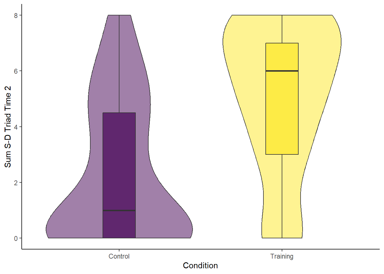
Across both time 1 and time 2, the group scores higher on average for the S-D triad measure.
The selection scores for both the Control and Training groups from time 1 to time 2.
This table calculates the mean and standard score for each variable per group. You can use this to answer the questions above.
| Condition | Variable | mean_score | sd_score |
|---|---|---|---|
| Control | SD_triad_time1 | 2.06 | 2.26 |
| Control | SD_triad_time2 | 2.33 | 2.57 |
| Control | selection_time1 | 1.69 | 0.97 |
| Control | selection_time2 | 1.18 | 0.89 |
| Training | SD_triad_time1 | 5.12 | 2.58 |
| Training | SD_triad_time2 | 5.10 | 2.67 |
| Training | selection_time1 | 2.33 | 1.34 |
| Training | selection_time2 | 1.90 | 1.37 |
- For our analyses, we are going to focus on each outcome in isolation to make the chapter accessible (but see the bonus analyses for when you are further in your studies). Create an appropriate plot to visualise the effect of
ConditiononSD_triad_time2, then do the same forselection_time2. Check your attempt against our example, but note there is creative freedom here providing it is appropriate for the variables.
The code here creates a violin-boxplot to visualise the difference in S-D Triad time 2 between the control and training groups.
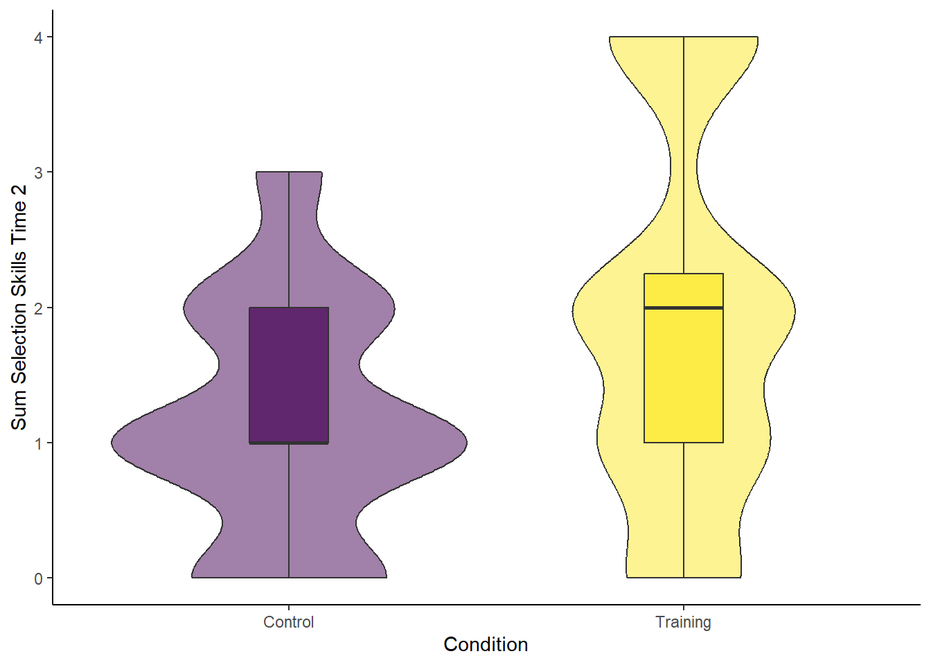
The code here creates a violin-boxplot to visualise the difference in selection skills time 2 between the control and training groups.
5.5 Analysis
Finally, we turn to analysis for inferential statistics. In Allen et al. (2021), they organise the analyses into three hypotheses:
“We hypothesized that, compared to untrained students, trained students would perform better on five tasks reflecting structural awareness”.
“We hypothesized that, compared to untrained students, trained students would demonstrate stronger statistic selection skills.”
“We hypothesized that these effects would be evident immediately following training (or a control task) and again following a 1-week delay”. You may not have developed all the analysis skills yet to reproduce their analyses exactly, so we will work around an adapted set.
We present each analysis as an overview so you can think about what techniques would address it, give you instructions on what analysis we have in mind if you need guidance, then present the solution. For the main guidance in this chapter, we are going to focus on each outcome and time point in isolation. The authors do this but they use something called Bayesian statistics which we do not cover on many courses, but you can see the resources in one of our other books (Statistics and Research Design) if you are curious).
At the end of the chapter, we provide some bonus examples for how you can approach the analysis to include all relevant variables, instead of focusing on group or time-point differences in isolation.
5.5.1 Hypothesis 1: Structural awareness
- Hypothesis 1 is that trained students will perform better on structural awareness tasks compared to untrained (control students). So, we expect participants in the Trained group to have higher S-D Triad scores at time 1 and time 2 compared to the Control group.
Identify an analysis technique that would address hypothesis 1. Remember the three key components of inferential statistics: hypothesis testing, a relevant effect size, and a relevant interval estimate. Does the example meet parametric assumptions?
To test whether the S-D Triad is higher in the Training group compared to the Control group at both time 1 and time 2, we need something that will handle a between-subjects design to compare two groups on one outcome. Something like simple linear regression to make the assumption checking easier, or a independent samples t-test.
Time 1
Fit the first model to include
Conditionas the predictor / IV andSD_triad_time1as the outcome / DV.Is the difference statistically significant? What is the effect size and confidence interval?
What do the model assumptions look like? Do you think this model is suitable for the data?
Time 2
Fit the first model to include
Conditionas the predictor / IV andSD_triad_time2as the outcome / DV.Is the difference statistically significant? What is the effect size and confidence interval?
What do the model assumptions look like? Do you think this model is suitable for the data?
Time 1
We first fit a simple linear regression model with Condition as the predictor / IV and SD_triad_time1 as the outcome.
Call:
lm(formula = SD_triad_time1 ~ Condition, data = allen_clean)

Residuals:
    Min      1Q  Median      3Q     Max
-5.1250 -2.0588 -0.0588  1.8750  5.9412

Coefficients:
                  Estimate Std. Error t value Pr(>|t|)
(Intercept)         2.0588     0.3389   6.076 2.42e-08 ***
ConditionTraining   3.0662     0.4867   6.300 8.71e-09 ***
---
Signif. codes:  0 '***' 0.001 '**' 0.01 '*' 0.05 '.' 0.1 ' ' 1

Residual standard error: 2.42 on 97 degrees of freedom
Multiple R-squared:  0.2904,    Adjusted R-squared:  0.2831
F-statistic:  39.7 on 1 and 97 DF,  p-value: 8.714e-09

                     2.5 %   97.5 %
(Intercept)       1.386263 2.731384
ConditionTraining 2.100285 4.032068
Consistent with hypothesis 1, participants in the Training group had higher structural awareness scores at time 1 than the Control group. On average, participants in the Training group scored 3.07 points (95% CI = [2.10, 4.03], p < .001) higher than the Control group.
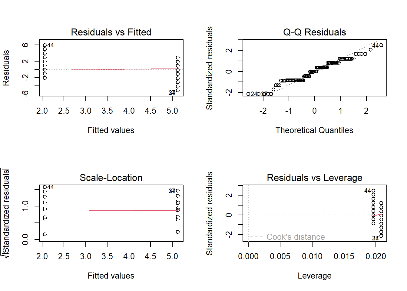
Checking the assumptions, the data looked a little suspect in the violin-boxplots earlier, but this is why it is important to check the model residuals, not the outcome itself. There are no major red flags here other than the qq plot suggests the data are somewhat discrete, with the scale points moving in steps as the values are only integers between 0 and 8.
Time 2
We first fit a simple linear regression model with Condition as the predictor / IV and SD_triad_time2 as the outcome.
Call:
lm(formula = SD_triad_time2 ~ Condition, data = allen_clean)

Residuals:
    Min      1Q  Median      3Q     Max
-5.1042 -2.3333 -0.1042  1.8958  5.6667

Coefficients:
                  Estimate Std. Error t value Pr(>|t|)
(Intercept)         2.3333     0.3669   6.360 6.62e-09 ***
ConditionTraining   2.7708     0.5269   5.259 8.63e-07 ***
---
Signif. codes:  0 '***' 0.001 '**' 0.01 '*' 0.05 '.' 0.1 ' ' 1

Residual standard error: 2.62 on 97 degrees of freedom
Multiple R-squared:  0.2219,    Adjusted R-squared:  0.2138
F-statistic: 27.66 on 1 and 97 DF,  p-value: 8.634e-07

                     2.5 %   97.5 %
(Intercept)       1.605210 3.061457
ConditionTraining 1.725146 3.816521
Consistent with hypothesis 1, participants in the Training group had higher structural awareness scores at time 2 than the Control group. On average, participants in the Training group scored 2.77 points (95% CI = [1.73, 3.82], p < .001) higher than the Control group.
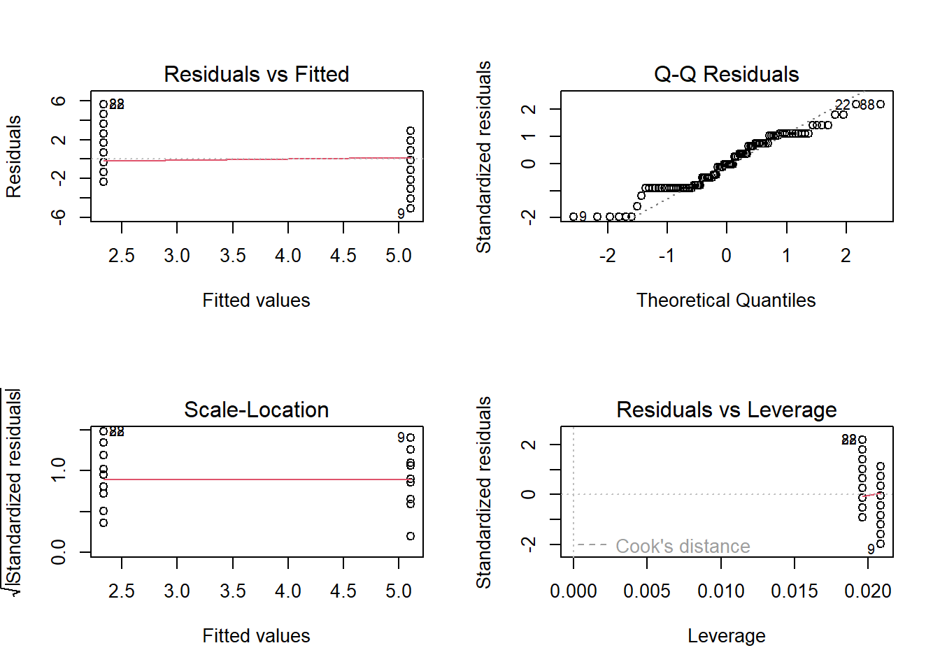
Checking the assumptions, the data look pretty similar to time 1. There are still no major red flags for our purposes here, but the qq plot looks worse than it did for time 1. We have a region around -1 on the x-axis where the scale points get stuck moving horizontally. If you look at the raw data, there are essentially fewer responses between 1 and 4 on the scale, than the other response options.
5.5.2 Hypothesis 2: Selection skills
- Hypothesis 2 is that trained students will perform better on selection skills compared to untrained (control students). So, we expect participants in the Trained group to have higher selection skill scores at time 1 and time 2 compared to the Control group.
Identify an analysis technique that would address hypothesis 2. Remember the three key components of inferential statistics: hypothesis testing, a relevant effect size, and a relevant interval estimate. Does the example meet parametric assumptions?
To test whether selection skills is higher in the Training group compared to the Control group at both time 1 and time 2, we need something that will handle a between-subjects design to compare two groups on one outcome. Something like simple linear regression to make the assumption checking easier, or a independent samples t-test.
Time 1
Fit the first model to include
Conditionas the predictor / IV andselection_time1as the outcome / DV.Is the difference statistically significant? What is the effect size and confidence interval?
What do the model assumptions look like? Do you think this model is suitable for the data?
Time 2
Fit the first model to include
Conditionas the predictor / IV andselection_time2as the outcome / DV.Is the difference statistically significant? What is the effect size and confidence interval?
What do the model assumptions look like? Do you think this model is suitable for the data?
Time 1
We first fit a simple linear regression model with Condition as the predictor / IV and selection_time1 as the outcome.
Call:
lm(formula = selection_time1 ~ Condition, data = allen_clean)

Residuals:
    Min      1Q  Median      3Q     Max
-2.3333 -0.6863  0.3137  0.6667  2.3137

Coefficients:
                  Estimate Std. Error t value Pr(>|t|)
(Intercept)         1.6863     0.1631  10.337  < 2e-16 ***
ConditionTraining   0.6471     0.2343   2.762  0.00687 **
---
Signif. codes:  0 '***' 0.001 '**' 0.01 '*' 0.05 '.' 0.1 ' ' 1

Residual standard error: 1.165 on 97 degrees of freedom
Multiple R-squared:  0.07291,   Adjusted R-squared:  0.06335
F-statistic: 7.628 on 1 and 97 DF,  p-value: 0.006874

                      2.5 %   97.5 %
(Intercept)       1.3625060 2.010043
ConditionTraining 0.1820817 1.112036
Consistent with hypothesis 2, participants in the Training group had higher selection skills at time 1 than the Control group. On average, participants in the Training group scored 0.65 points (95% CI = [0.18, 1.11], p = .007) higher than the Control group.
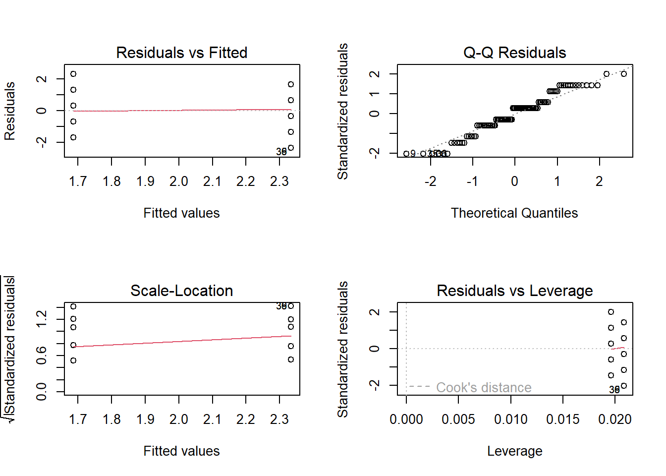
Checking the assumptions, the data follow a similar pattern to SD Triad time 1. There are no major red flags here other than the qq plot suggests the data are somewhat discrete, with the scale points moving in steps as the values are only integers between 0 and 4.
Time 2
We first fit a simple linear regression model with Condition as the predictor / IV and selection_time2 as the outcome.
Call:
lm(formula = selection_time2 ~ Condition, data = allen_clean)

Residuals:
    Min      1Q  Median      3Q     Max
-1.8958 -0.8958 -0.1765  0.8235  2.1042

Coefficients:
                  Estimate Std. Error t value Pr(>|t|)
(Intercept)         1.1765     0.1608   7.317 7.36e-11 ***
ConditionTraining   0.7194     0.2309   3.115  0.00242 **
---
Signif. codes:  0 '***' 0.001 '**' 0.01 '*' 0.05 '.' 0.1 ' ' 1

Residual standard error: 1.148 on 97 degrees of freedom
Multiple R-squared:  0.09095,   Adjusted R-squared:  0.08158
F-statistic: 9.705 on 1 and 97 DF,  p-value: 0.002417

                      2.5 %   97.5 %
(Intercept)       0.8573544 1.495587
ConditionTraining 0.2610670 1.177659
Consistent with hypothesis 2, participants in the Training group had higher selection skills at time 2 than the Control group. On average, participants in the Training group scored 0.72 points (95% CI = [0.26, 1.18], p = .002) higher than the Control group.
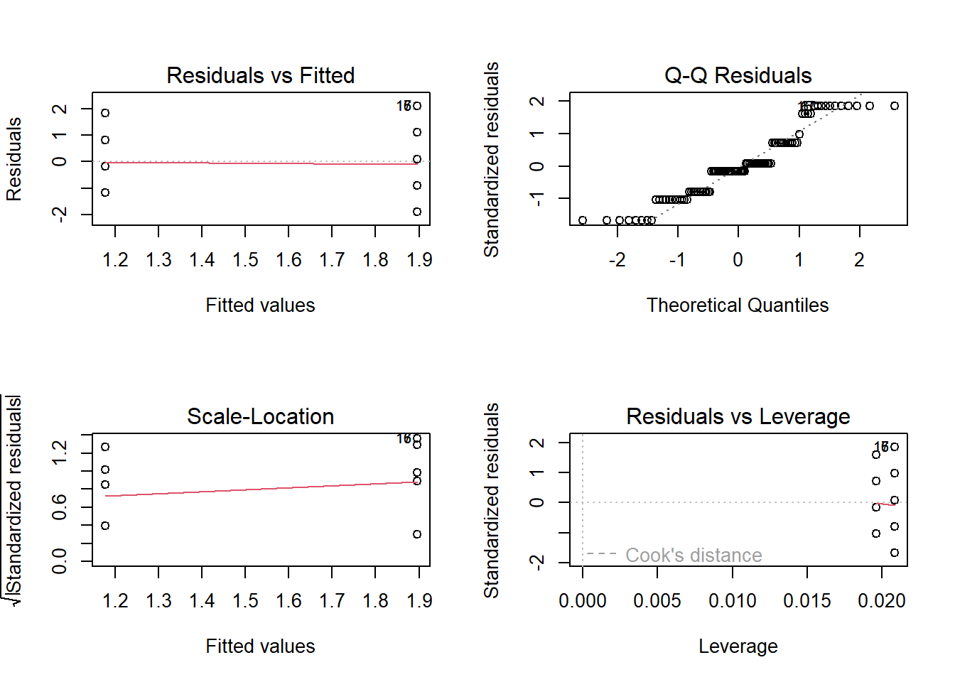
Checking the assumptions, the data look pretty similar to time 1. There are still no major red flags for our purposes here apart from the integer data.
5.5.3 Bonus analysis: 2x2 Mixed ANOVA
One alternative is to include the interaction between Condition and Time in one model. This will address both the group and time element, to investigate if the difference between the groups has a different magnitude across the two time-points (or the opposite: whether the difference between time-points has a different magnitude across the two groups).
Restructure the data to pivot the data longer, where
SD_triad_time1andSD_triad_time2are now two rows per participant. Name the new columns something likeTimefor time 1 and time 2, andResponsefor the value of the outcome per observation.Fit a 2x2 mixed ANOVA to test the main effects of
ConditionandTime, and their interaction. Are any effects statistically significant? How can you calculate a relevant effect size?How can you visualise the full design?
In the code below, we need three packages for the bonus sections, then we restructure the data to spread S-D Triad across two rows - one for each time-point. We then fit a 2x2 mixed ANOVA.
library(afex)
library(sjPlot)
library(emmeans)

# Step 1 - Restructure the data for long-form time
allen_long <- allen_clean %>%
  pivot_longer(cols = SD_triad_time1:SD_triad_time2,
               names_to = "Time",
               values_to = "Response")

SD_triad_ANOVA <- aov_ez(id = "ID",
                         dv = "Response",
                         data = allen_long,
                         between = "Condition",
                         within = "Time",
                         type = 3,
                         # partial eta squared
                         anova_table = list(es = "pes"))

SD_triad_ANOVA
Anova Table (Type 3 tests)
Response: Response
Effect df MSE F pes p.value
1 Condition 1, 97 11.13 37.86 *** .281 <.001
2 Time 1, 97 1.59 0.50 .005 .482
3 Condition:Time 1, 97 1.59 0.68 .007 .413
---
Signif. codes: 0 '***' 0.001 '**' 0.01 '*' 0.05 '+' 0.1 ' ' 1The results are broadly consistent with the simple / t-test approach in the main part of the chapter. There is a significant main effect of Condition, meaning there is an overall significant difference between Training and Control. There is not a significant main effect of Time, and there is no significant interaction between Condition and Time.
We can understand this a little better by visualising things. We add between-subjects confidence intervals to compare the two groups rather than within-subjects.
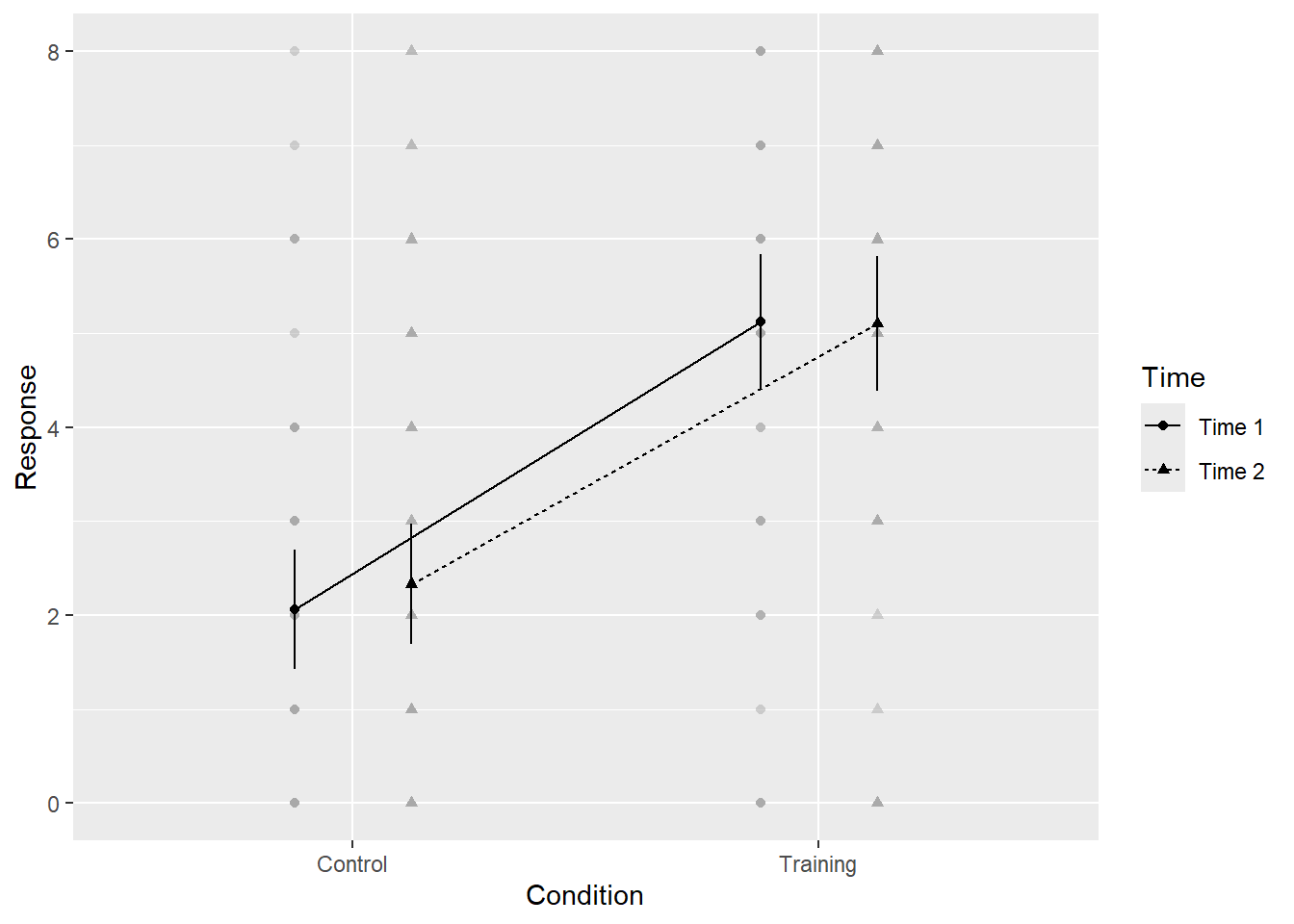
We can see pretty clearly how Training consistently scores higher on S-D Triad than Control. The lines are roughly parallel, showing how the effect is somewhat constant from time 1 to time 2.
We can also calculate an effect size to summarise the estimated marginal mean difference between Control and Training groups, given this was the significant main effect.
$emmeans
 Condition emmean   SE df lower.CL upper.CL
 Control     2.20 0.33 97     1.54     2.85
 Training    5.11 0.34 97     4.44     5.79

Results are averaged over the levels of: Time
Confidence level used: 0.95

$contrasts
 contrast           estimate    SE df t.ratio p.value
 Control - Training    -2.92 0.474 97  -6.153  <.0001

Results are averaged over the levels of: Time
5.5.4 Bonus analysis: ANCOVA regression
A pre-test post-test design like this is very common in research (particularly clinical trials) and there are lots of discussions among statisticians for what is the most effective way of modelling the effects. We worked through a 2x2 mixed ANOVA (you could also fit a mixed effects model to stick with the regression format), but one underused approach in psychology is an ANCOVA approach. Instead of calculating something like a difference score (time 2 - time 1) and comparing between groups, you use time 2 as the outcome, then time 1 and group as individual predictors.
Create a new variable to center (substract each observation from the mean)
selection_time1. To make things easier later, make sureConditionis a factor.Fit a multiple regression model using
selection_time2as the outcome, with your new centeredselection_time1andConditionas two individual predictors (no interaction).Is the effect of
Conditionstatistically significant? What is the effect size and confidence interval?How can you visualise the effect?
In the code below, we first create a new variable selection_time1_center to center selection_time1. We then fit the multiple regression model.
allen_center <- allen_clean %>%
  mutate(selection_time1_center = selection_time1 - mean(selection_time1),
         Condition = as.factor(Condition))

selection_covar_model <- lm(selection_time2 ~ selection_time1_center + Condition,
                            data = allen_center)

summary(selection_covar_model)

confint(selection_covar_model)
Call:
lm(formula = selection_time2 ~ selection_time1_center + Condition,
    data = allen_center)

Residuals:
    Min      1Q  Median      3Q     Max
-2.5730 -0.6416 -0.1667  0.6961  2.2396

Coefficients:
                       Estimate Std. Error t value Pr(>|t|)
(Intercept)             1.30394    0.15003   8.691 9.60e-14 ***
selection_time1_center  0.40632    0.09165   4.433 2.47e-05 ***
ConditionTraining       0.45645    0.21963   2.078   0.0404 *
---
Signif. codes:  0 '***' 0.001 '**' 0.01 '*' 0.05 '.' 0.1 ' ' 1

Residual standard error: 1.052 on 96 degrees of freedom
Multiple R-squared:  0.2454,    Adjusted R-squared:  0.2297
F-statistic: 15.61 on 2 and 96 DF,  p-value: 1.347e-06

                            2.5 %    97.5 %
(Intercept)            1.00613390 1.6017501
selection_time1_center 0.22439103 0.5882393
ConditionTraining      0.02049321 0.8924127
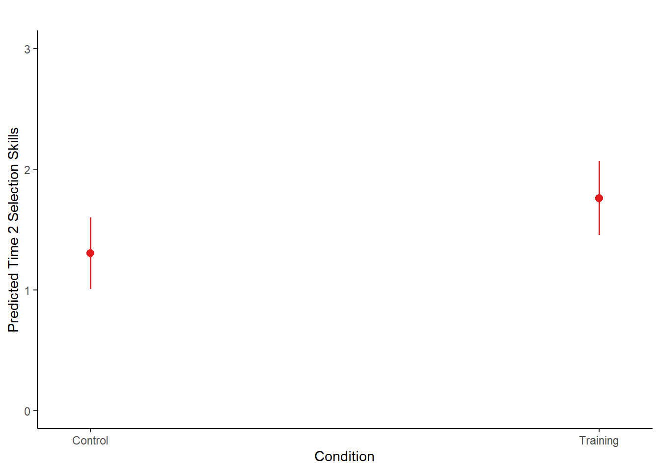
The predictor we are interested in is ConditionTraining. This is like the main example where we estimate the difference between Control (the intercept/reference group) and Training. Here it is statistically significant, where those in the Training group score 0.46 (95% CI = [0.02, 0.89], p = .040) points higher on average compared to the control group. For the interpretation though, this is a partial effect where it is “controlling” for the effect of selection skills at time 1. The selection_time1_center predictor itself is rarely of interest as pre-test covariates like this will almost always be significant as time 1 and time 2 scores from the same participant tend to be heavily correlated.
Finally, we can plot the partial effect to visualise the partial effect.
5.6 Conclusion
Well done! Hopefully you recognised how far your skills have come to be able to do this independently, regardless of how many hints you needed. If you are curious, you can read Allen et al. (2021) to see how they analyse and visualise the data.
Like the bonus analyses show, there are often competing ways of modelling the data. The main thing to keep in mind is that you want to address your research question / hypothesis, and you are trying to identify the statistical test that will help you given the design/data you have available.
There are more alternatives we have not demonstrated here, like a mixed effects model, or even ordinal regression given the discrete outcomes. There are always decisions to make, you job is to be as clear and honest as possible about why you chose the approach you did given alternatives.