2 Pennington et al. (2026): Awareness and Use of Open Research Practices
In this chapter, we assume you have covered data wrangling tasks such as selecting variables, joining datasets, creating and modifying variables, and calculating summary statistics. There are then some basic visualisation opportunities to create things like bar plots.
2.1 Task preparation
2.1.1 Introduction to the data set
For this task, we are using open data from Pennington et al. (2026). The abstract of their article is:
Background: Growing concerns about replicability, reproducibility, and transparency have led to the adoption of several open research practices aimed at reforming the academic ecosystem. The current study explores international researcher’s awareness and use of open research practice and variations across regions, disciplines, methodologies, and career level. Methods: A total of 3,017 researchers (45 countries; 24 disciplines) completed the Brief Open Research Survey, reporting their awareness and use of eleven common open research practices and factors that would support their adoption. Results: Respondents reported high awareness of Open Access Publishing, Preprints, and Open Data and awareness only fell below 50% for Research Co-production and Registered Reports. Use was high for Open Access Publishing, but fell below 50% for Preprints, Open Data, Open Research [term], Open Materials, Open Peer Review, Open Code, Preregistration, Research Co-production, Replication, and Registered Reports. Awareness and use varied across the sampled regions (e.g., Europe vs. Asia), disciplines (e.g., Psychology vs. General & Others in Sciences), methodologies (e.g., quantitative vs. qualitative), and career stages (e.g., PhD students vs. Professors). Respondents reported that the top five supportive strategies of open research were incentives from funders, institutions and regulators; dedicated funding; recognition in promotion and recruitment criteria; more training; and more information. Conclusions: Awareness is uniformly higher than use across open research practices and there are important variations between regions, methodologies, and career stages, as well as discipline-specific practices.
To summarise, they were interested in measuring the awareness and usage gap in common open science practices. Pennington et al. presented 3017 researchers with these practices and recorded several demographic variables. To avoid triangulation, the researchers separated the data into several files. We can describe their research question as: “What is the prevalence of awareness and use of common open research practices across international regions?”. For this chapter, we will summarise and visualise the data to look for patterns across the whole sample and across countries.
2.1.2 Organising your files and project for the task
Before we can get started, you need to organise your files and project for the task, so your working directory is in order.
You can create a folder for the data analysis journeys book and a new sub-folder for this chapter, something like:
analysis_journeys, create a new folder for this chapter called something likePennington_wrangling. WithinPennington_wrangling, create two new folders calleddataandfigures.Create an R Project for
Pennington_wranglingas an existing directory for your chapter folder. This should now be your working directory.Create a new Quarto document and give it a sensible title describing the chapter, such as
Pennington et al. (2026): Data Wrangling. Delete everything below line 10 so you have a blank file to work with and save the file in yourPennington_wranglingfolder.You can download the country data file (Pennington_country.csv) here. Right click the link and select “save link as”, or clicking the link will save the file to your Downloads. Make sure that you save the file as “.csv”. Save or copy the file to your
data/folder withinPennington_wrangling.
You are now ready to start working on the task!
2.2 Overview
2.2.1 Load tidyverse and read the data file
Before we explore what wrangling we need to do, load
2.2.2 Explore country
In country, we have the participant ID (ID) , data quality items, which country the researcher came from, 11 items for awareness of open research practices, and 11 items for usage of open research practices. The columns (variables) we have in the data set are:
| Variable | Type | Description |
|---|---|---|
id |
character | Participant ID number. |
finished |
logical | Whether the participant finished the study; TRUE = yes, FALSE = no. |
consent |
character | Whether the participant consented; Yes or No. |
country |
character | The country of origin for the participant from drop-downs. |
country_analysis |
character | The country of origin for the participants, combining free-text option. |
aware_open_research to aware_research_co_production
|
character | 11 items for awareness, with responses of “I’m aware of this” or NA. |
used_open_research to used_research_co_production
|
character | 11 items for usage, with responses of “I’ve used this”, “I’ve not used this”, “Not applicable to my research”, or NA. |
Now we have introduced the data set, explore it using different methods we introduced. For example, opening the data object as a tab to scroll around, explore with glimpse(), or even try plotting some of the variables to see what they look like.
Remember, their research question was: “What is the prevalence of awareness and use of common open research practices across international regions?”. After reading the code book and exploring the initial data, what steps do you think you will need to take to wrangle the data to be able to answer this question?
2.3 Wrangling the data
Before we start wrangling the awareness and usage data, we can check some details of the countries. For example, how many countries are included in the data, what are the most and least frequent countries? Fortunately, the survey used drop-down boxes, so we do not have to worry about nasty free-text shenanigans.
Remember: you might not use the exact same code as our solutions, it is getting the correct answer which is important. Sometimes our code will be more efficient and you can learn some new tricks, other times you might have a more elegant solution than us.
- How many countries are included in the data (use
country_analysisto get the full list)? There were unique countries, excluding NA responses.
- What was the most frequent response country (use
country_analysisto get the full list)? The most frequent response country was .
- How many countries only had one respondent (using
country_analysis)? There were countries with only one respondent.
2.3.1 Wrangling awareness and usage
Now that we have had a little explore of the country variables, it is time to wrangle the awareness and usage data into something we can get insights from. As a reminder, the research question was “What is the prevalence of awareness and use of common open research practices across international regions and disciplines?”. We need to wrangle the data to be able to address the international regions element of the research question, so ask yourself how we can work with the variables to estimate the prevalence of awareness and usage by country. If you look at the original paper by Pennington et al., they code the data into four categories: used, not used: aware, not used: unaware, and not applicable. So, this will be our first challenge.
We are going to show you a preview of the starting data set and the end product we are aiming for.
Rows: 3,017
Columns: 27
$ id                            <chr> "P1", "P2", "P3", "P4", "P5", "P6", "P7"…
$ finished                      <lgl> TRUE, TRUE, TRUE, TRUE, TRUE, TRUE, TRUE…
$ consent                       <chr> "Yes", "Yes", "Yes", "Yes", "Yes", "Yes"…
$ country                       <chr> "United Kingdom", "Australia", "United K…
$ country_analysis              <chr> "United Kingdom", "Australia", "United K…
$ aware_open_research           <chr> "I'm aware of this", "I'm aware of this"…
$ aware_study_preregistration   <chr> "I'm aware of this", "I'm aware of this"…
$ aware_registered_reports      <chr> "I'm aware of this", "I'm aware of this"…
$ aware_open_materials          <chr> NA, "I'm aware of this", "I'm aware of t…
$ aware_open_data               <chr> "I'm aware of this", "I'm aware of this"…
$ aware_open_code               <chr> "I'm aware of this", "I'm aware of this"…
$ aware_preprints               <chr> "I'm aware of this", "I'm aware of this"…
$ aware_open_peer_review        <chr> "I'm aware of this", "I'm aware of this"…
$ aware_open_access_publication <chr> "I'm aware of this", "I'm aware of this"…
$ aware_replication_studies     <chr> "I'm aware of this", "I'm aware of this"…
$ aware_research_co_production  <chr> NA, NA, NA, NA, "I'm aware of this", "I'…
$ used_open_research            <chr> "I've used this", "I've used this", "I'v…
$ used_study_preregistration    <chr> "I've not used this", "I've used this", …
$ used_registered_reports       <chr> "I've not used this", "I've used this", …
$ used_open_materials           <chr> NA, "I've used this", "I've used this", …
$ used_open_data                <chr> "I've used this", "I've used this", "I'v…
$ used_open_code                <chr> "I've used this", "I've used this", "I'v…
$ used_preprints                <chr> "I've used this", "I've used this", "I'v…
$ used_open_peer_review         <chr> "Not applicable to my research", "I've u…
$ used_open_access_publication  <chr> "I've used this", "I've used this", "I'v…
$ used_replication_studies      <chr> "I've used this", "I've used this", "I'v…
$ used_research_co_production   <chr> NA, NA, NA, NA, "I've not used this", "I…
Rows: 33,187
Columns: 9
$ id <chr> "P1", "P1", "P1", "P1", "P1", "P1", "P1", "P1", "P1",…
$ finished <lgl> TRUE, TRUE, TRUE, TRUE, TRUE, TRUE, TRUE, TRUE, TRUE,…
$ consent <chr> "Yes", "Yes", "Yes", "Yes", "Yes", "Yes", "Yes", "Yes…
$ country <chr> "United Kingdom", "United Kingdom", "United Kingdom",…
$ country_analysis <chr> "United Kingdom", "United Kingdom", "United Kingdom",…
$ practice <chr> "open_research", "study_preregistration", "registered…
$ awareness <chr> "I'm aware of this", "I'm aware of this", "I'm aware …
$ usage <chr> "I've used this", "I've not used this", "I've not use…
$ experience <chr> "Used", "Not used: Aware", "Not used: Aware", "Not us…Before we give you a task list, try and switch between the raw data and the wrangled data. Make a list of all the differences you can see between the two data objects.
What type is each variable? Has it changed from the raw data?
Do we have any new variables? How could you create these from the variables available to you?
For the variable experience, this has four options which you cannot see in the preview: “Used”, “Not used: Aware”, “Not used: Unaware”, and “N/A to my research”. Which variable(s) could this be based on?
- Do any variables look like they have been restructured? Do you need to pivot anything longer or wider?
Try and wrangle the data based on all the differences you notice to create a new object usage_practices.
When you get as far as you can, check the task list which explains all the steps we applied, but not how to do them. Then, you can check the solution for our code. When we start the summarising stage, we will need some additional smaller wrangling steps, but this will represent the bulk of the work.
2.3.1.1 Task list
These are all the steps we applied to create the wrangled data object usage_practices:
Create a new object called
usage_practicesfrom the original objectcountry. You can either create multiple objects as you go or create one long pipe chain from this point.Pivot longer to turn the data into long-form. Select all the awareness and usage columns from
aware_open_researchtoused_research_co_production. Label the names as “practice” for open science practices and label the values as “response” for their response.Currently,
practiceincludes the different practices twice: once for awareness and once for usage. We need a couple of steps to turn this into data that is easier to work with. Mutate to add a new column called “usage” which labels each row inpracticeas “awareness” and “usage”.
Hint: The grepl() function can look for text patterns to create a logical variable.
- Mutate to overwrite the
practicevariable. Now that we have created our newusagevariable, we want to remove the “aware_” and “used_” prefixes. For each row inpractice, we only want the practice itself, such as “open_research”, not “awareness_open_research”.
Hint: The sub() function can substitute text if you give it a pattern to look for and what you want to replace it with (e.g., nothing).
Now that we have tidied up
practiceand created ourusagevariable, we need some restructuring. Pivot the data wider to keep all the columns fromidtopractice, but move theusagevariable to new column names and use theresponsevariable for values.-
Now that there are two columns for
awarenessandusage, we want to mutate and add a new variable calledexperience, coding for one of four responses:Used
Not used: Aware
Not used: Unaware
“N/A to my research.
Hint: Use something like case_when() to create a variable based on combinations of awareness and usage.
For some advice, think of everything you have covered so far in your course book. How could you complete these steps as efficiently as possible? Could you string together functions using pipes, or do you need some intermediary objects? If it’s easier for you to complete steps with longer but accurate code, there is nothing wrong with that. You recognise ways to make your code more efficient over time.
2.3.1.2 Solution
This is the code we used to create the new object usage_practices using the original object country. As long as you get the same end result, the exact code is not important. In coding, there are multiple ways of getting to the same end result. Maybe you found a more efficient way to complete some of the steps compared to us. Maybe your code was a little longer. As long as it worked, that is the most important thing.
# create an overall object called usage_practices
usage_practices <- country %>%
  # pivot longer using all the awareness and usage variables
  pivot_longer(cols = aware_open_research:used_research_co_production,
               names_to = "practice",
               values_to = "response") %>%
  # add a new column usage for whether the practice is awareness or usage
  mutate(usage = case_when(grepl("aware_", practice) ~ "awareness",
                           grepl("used_", practice) ~ "usage"),
         # edit the practice variable to remove the aware_ and used_ prefixes
         practice = sub("aware_", "", practice),
         practice = sub("used_", "", practice)) %>%
  # pivot wider usage and response, ignoring all the other variables
  pivot_wider(id_cols = id:practice,
              names_from = usage,
              values_from = response) %>%
  # create an experience variable for the four combinations of interest
  mutate(experience = case_when(awareness == "I'm aware of this" & usage == "I've used this" ~ "Used",
                                awareness == "I'm aware of this" & usage == "I've not used this" ~ "Not used: Aware",
                                is.na(awareness) ~ "Not used: Unaware",
                                usage == "Not applicable to my research" ~ "N/A to my research"))
2.4 Summarising and visualising the data
Now that we have wrangled the data mostly into shape, we can start to ask some questions. If you look at the original paper by Pennington et al., they first look at patterns across the whole sample, and then by region. So, for each element, we will need a couple of smaller wrangling steps.
2.4.1 Open research practices overall
Before we start asking questions of the total sample, we need a small wrangling step to generate percentages per practice and experience. Create a new object called count_sample using the usage_practices object. Count the frequencies of the combination of practice and experience variables, then calculate the percentage of respondents out of the total sample size, rounding to floor (floor()) to avoid rounding errors. Check your code against the solution when you have attempted it yourself first.
Now you have completed the final wrangling step, try and answer the following questions. Complete the interactive questions and check your answers against the solution code if you are stuck.
- Imagine you wanted to help other early career researchers develop their open research skills. However, you can only run so many sessions and you need to identify the biggest priority. Out of all the open research practices, which one had the highest response rate for “Not used: unaware”? The highest unawareness category was for: .
| practice | experience | n | percentage |
|---|---|---|---|
| registered_reports | Not used: Unaware | 1737 | 57 |
| research_co_production | Not used: Unaware | 1599 | 52 |
| study_preregistration | Not used: Unaware | 1484 | 49 |
| open_code | Not used: Unaware | 1180 | 39 |
| replication_studies | Not used: Unaware | 1086 | 35 |
| open_materials | Not used: Unaware | 983 | 32 |
| open_peer_review | Not used: Unaware | 906 | 30 |
| open_research | Not used: Unaware | 883 | 29 |
| open_data | Not used: Unaware | 657 | 21 |
| preprints | Not used: Unaware | 594 | 19 |
| open_access_publication | Not used: Unaware | 229 | 7 |
- As part of a group presentation, you need to visualise the open research practices to show the usage rates. Recreate the following bar plot to show the percentage of respondents who have used a given open science practice (we will ignore tidying up the practice labels for these exercises).
Hint: If you have not learnt how to flip axes, check out the coord_flip() function.
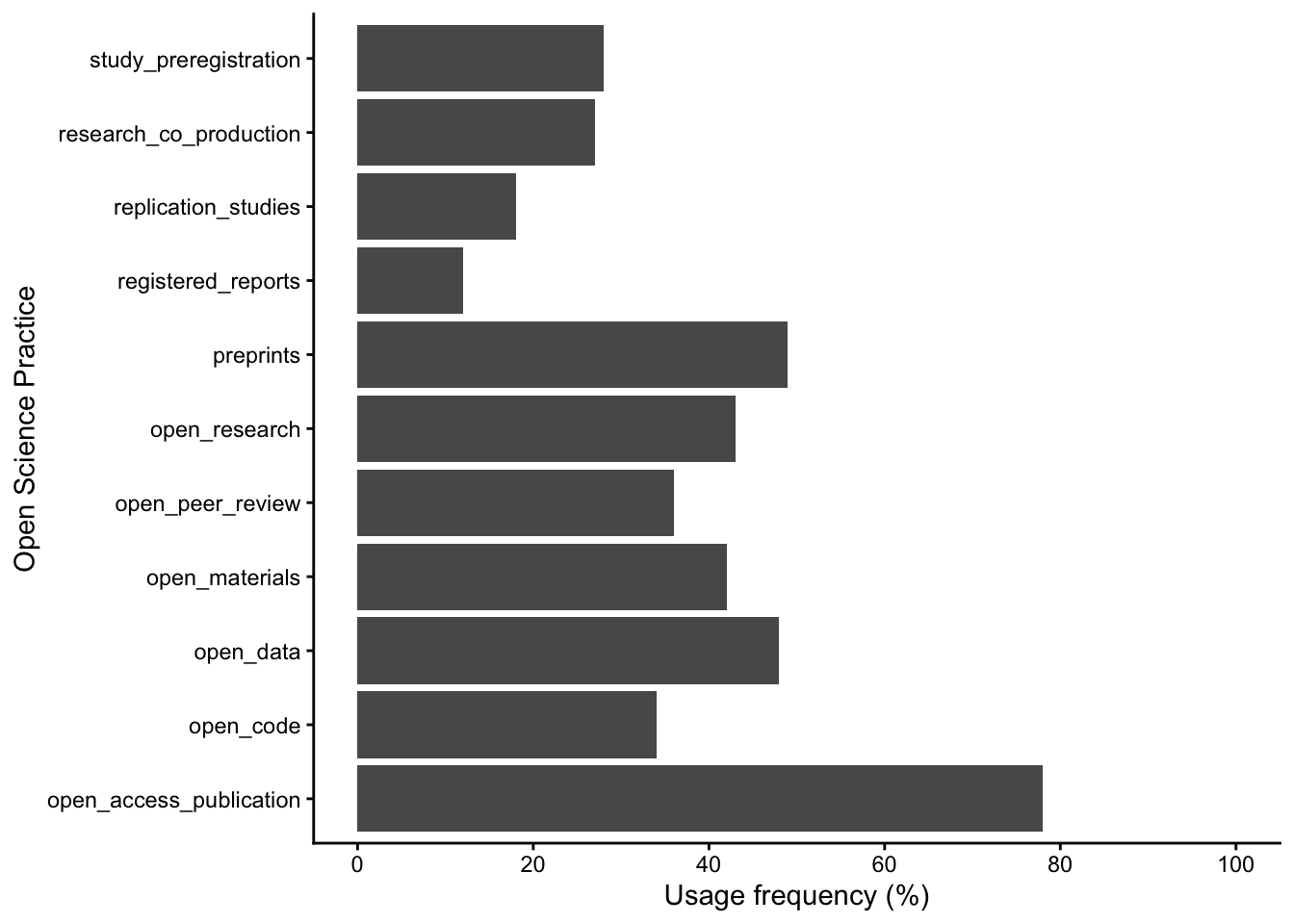
count_sample %>%
  filter(experience == "Used") %>%
  ggplot(aes(x = practice, y = percentage)) +
  geom_bar(stat = "identity") +
  coord_flip() +
  theme_classic() +
  scale_x_discrete(name = "Open Science Practice") +
  scale_y_continuous(name = "Usage frequency (%)",
                     breaks = seq(0, 100, 20),
                     limits = c(0, 100))
- One potential danger in promoting or mandating open research practices is that it is not applicable or suitable to people’s research discipline. Looking at the different practices, this reassuringly does not seem to be the case, with a prevalence percentage ranging between % and %.
| practice | experience | n | percentage |
|---|---|---|---|
| open_access_publication | N/A to my research | 36 | 1 |
| open_code | N/A to my research | 243 | 8 |
| open_data | N/A to my research | 137 | 4 |
| open_materials | N/A to my research | 136 | 4 |
| open_peer_review | N/A to my research | 37 | 1 |
| open_research | N/A to my research | 91 | 3 |
| preprints | N/A to my research | 48 | 1 |
| registered_reports | N/A to my research | 70 | 2 |
| replication_studies | N/A to my research | 164 | 5 |
| research_co_production | N/A to my research | 60 | 1 |
| study_preregistration | N/A to my research | 110 | 3 |
- As a bonus task to this section, we can try and recreate their Figure 4 as close as we can without editing minor details. There might be some techniques in here which are unfamiliar to you, so do your best to find solutions yourself before you check the code. We have a stacked bar plot ordered by the open science practice being most frequent in the “Used” category from the top.
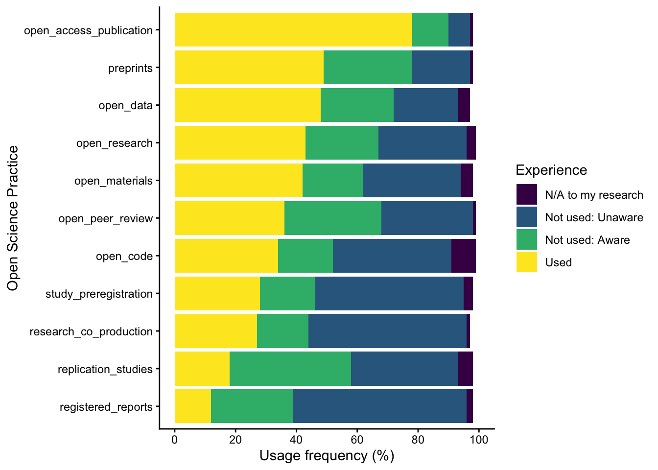
order_practices <- count_sample %>%
  filter(experience == "Used") %>%
  arrange(percentage)

count_sample %>%
  mutate(experience = factor(experience,
                             levels = c("N/A to my research", "Not used: Unaware", "Not used: Aware", "Used")),
         practice = factor(practice, levels = order_practices$practice)) %>%
  ggplot(aes(x = practice, y = percentage, fill = experience)) +
  geom_bar(stat = "identity") +
  coord_flip() +
  theme_classic() +
  scale_x_discrete(name = "Open Science Practice") +
  scale_y_continuous(name = "Usage frequency (%)",
                     breaks = seq(0, 100, 20),
                     limits = c(0, 100)) +
  scale_fill_viridis_d(name = "Experience")
2.4.2 Open research practices by region
Now that we have explored the overall patterns, we can address their research question more directly to explore prevalence across international regions. We will diverge from the original paper a little at this point to avoid grouping the countries into continental regions, but you are more than welcome to try and reproduce their percentages and Figure 5 yourself.
First, we need some additional wrangling. We do not want to calculate the percentages across the whole sample, we want to calculate percentages by country. We cannot use the total sample size as the denominator this time, we need the sample size per country first.
As the first step, create a new object called country_responses using the usage_practices object. You want to count the frequency of responses for the country_analysis variable. Then, rename the frequency as total_N.
As the second step, create a new object called count_countries using the usage_practices object:
Count the frequencies of the combination of
country_analysis,practiceandexperiencevariables.Join the two objects (
country_responsesandcount_countries) together bycountry_analysis, and you should now have both a sample size (n) per country, practice, and experience, and the total sample size per country.Calculate the percentage of respondents per experience out of the sample size per country, rounding to floor (
floor()) to avoid rounding errors.Finally, there are some countries with very few responses, so filter
total_Nto only include countries with 20 or more participants.
Check your code against the solution when you have attempted it yourself first.
# count the number of respondents per country
# we need this for percentages later
country_responses <- country %>%
  count(country_analysis) %>%
  rename(total_N = n)

count_countries <- usage_practices %>%
  count(country_analysis, practice, experience) %>%
  full_join(country_responses,
            by = "country_analysis") %>%
  mutate(percentage = floor((n / total_N*100))) %>%
filter(total_N >= 20)Now that you have completed the final wrangling steps, we have a few more questions for you to practice your summarising and visualising skills. Complete the interactive questions and check your answers against the solution code if you are stuck.
- After applying our exclusion criteria of removing countries with fewer than 20 participants, how many unique countries remain in the data set? There are countries remaining in
count_countries.
- We are not replicating the Pennington et al. analyses fully as they group the countries into continents, but we will ask similar questions. Which country has the highest and lowest awareness (combining “Used” and “Not used: Aware”) rate for open access publications? The highest awareness rate was in and the lowest awareness rate was in .
| country_analysis | sum_percentage |
|---|---|
| Japan | 99 |
| United States | 99 |
| Sweden | 97 |
| Switzerland | 96 |
| Netherlands | 95 |
| Norway | 95 |
| Finland | 94 |
| Germany | 93 |
| Australia | 92 |
| Italy | 92 |
| Austria | 91 |
| Belgium | 90 |
| Croatia | 90 |
| Slovakia | 90 |
| United Kingdom | 89 |
| Chile | 87 |
| Turkey | 87 |
| Brazil | 80 |
| Tanzania | 66 |
-
Focusing on practices that the majority of respondents in a country are unaware of (“Not used: Unaware”), fill in the blanks for the countries and practices that require the most support:
Country: Chile - Practice: - Percentage unaware: 92%.
Country: - Practice: Registered reports - Percentage unaware: 80%.
Country: Slovakia - Practice: Pre-registration - Percentage unaware: %.
| country_analysis | practice | experience | n | total_N | percentage |
|---|---|---|---|---|---|
| Chile | study_preregistration | Not used: Unaware | 37 | 40 | 92 |
| Belgium | registered_reports | Not used: Unaware | 16 | 20 | 80 |
| Tanzania | study_preregistration | Not used: Unaware | 26 | 34 | 76 |
| Belgium | study_preregistration | Not used: Unaware | 15 | 20 | 75 |
| Slovakia | study_preregistration | Not used: Unaware | 202 | 271 | 74 |
| Turkey | open_research | Not used: Unaware | 26 | 35 | 74 |
- Finally, Pennington et al. were interested in the usage rates for open access publications across countries. Recreate the following bar plot as close as possible to visualise the usage percentage from highest to lowest.
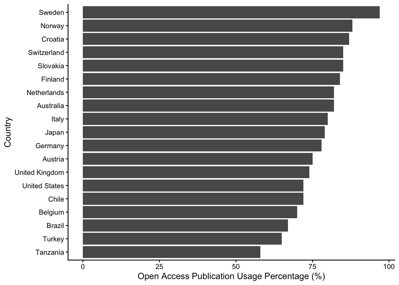
order_countries <- count_countries %>%
  filter(practice == "open_access_publication", experience == "Used") %>%
  arrange(percentage)

count_countries %>%
  filter(practice == "open_access_publication", experience == "Used") %>%
  mutate(country_analysis = factor(country_analysis,
                                   levels = order_countries$country_analysis)) %>%
  ggplot(aes(x = country_analysis, y = percentage)) +
  geom_bar(stat = "identity") +
  theme_classic() +
  coord_flip() +
  scale_y_continuous(name = "Usage Percentage (%)") +
  scale_x_discrete(name = "Country")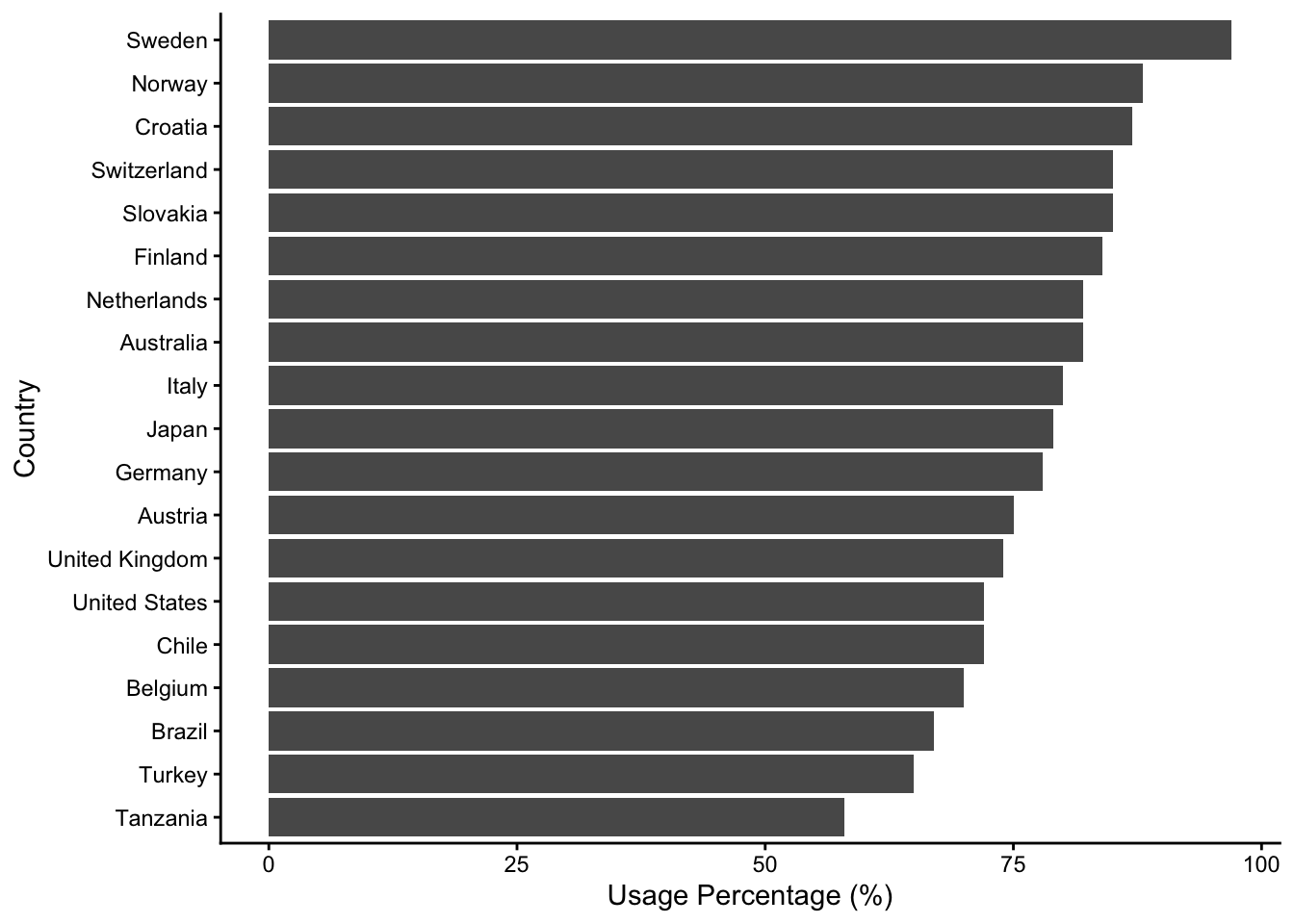
2.5 Conclusion
Well done on completing these activities! We hope you enjoyed practicing your wrangling and visualisation skills. It does not matter how many times you had to check the solution, you practiced your skills on a new scenario. Over time, you will get faster at recognising the wrangling steps you need to apply to your data to answer your research questions.