5 Data wrangling 1
So far you have been introduced to the R environment (e.g. setting
your working directory and the difference between .R and .Rmd files).
You also began working with messy data by having a go at loading in
datasets using read_csv(), joined files together using
inner_join(), and pulled out variables of interest using
select().
In this chapter, we'll be moving on to becoming familiar with the
Wickham Six and the functionality of the R package,
tidyverse!
Data comes in lots of different formats. One of the most common formats is that of a two-dimensional table (the two dimensions being rows and columns). Usually, each row stands for a separate observation (e.g. a subject), and each column stands for a different variable (e.g. a response, category, or group). A key benefit of tabular data (i.e., data in a table) is that it allows you to store different types of data-numerical measurements, alphanumeric labels, categorical descriptors-all in one place.
It may surprise you to learn that scientists actually spend far more time cleaning and preparing their data than they spend actually analysing it. This means completing tasks such as cleaning up bad values, changing the structure of tables, merging information stored in separate tables, reducing the data down to a subset of observations, and producing data summaries. Some have estimated that up to 80% of time spent on data analysis involves such data preparation tasks (Dasu & Johnson, 2003)!
Many people seem to operate under the assumption that the only option for data cleaning is the painstaking and time-consuming cutting and pasting of data within a spreadsheet program like Excel. We have witnessed students and colleagues waste days, weeks, and even months manually transforming their data in Excel, cutting, copying, and pasting data. Fixing up your data by hand is not only a terrible use of your time, but it is error-prone and not reproducible. Additionally, in this age where we can easily collect massive datasets online, you will not be able to organise, clean, and prepare these by hand.
In short, you will not thrive as a psychologist if you do not learn some key data wrangling skills. Although every dataset presents unique challenges, there are some systematic principles you should follow that will make your analyses easier, less error-prone, more efficient, and more reproducible.
In this chapter you will see how data science skills will allow you to efficiently get answers to nearly any question you might want to ask about your data. By learning how to properly make your computer do the hard and boring work for you, you can focus on the bigger issues.
5.1 Tidyverse
Tidyverse (https://www.tidyverse.org/) is a collection of R packages created by world-famous data scientist Hadley Wickham.
Tidyverse contains six core packages: dplyr, tidyr, readr, purrr, ggplot2, and tibble. In the last chapter when you typed library(tidyverse) into R, you will have seen that it loads in all of these packages in one go. Within these six core packages, you should be able to find everything you need to wrangle and visualise your data.
In this chapter, we are going to focus on the dplyr package, which contains six important functions:
-
select()Include or exclude certain variables (columns) -
filter()Include or exclude certain observations (rows) -
mutate()Create new variables (columns) -
arrange()Change the order of observations (rows) -
group_by()Organize the observations into groups -
summarise()Derive aggregate variables for groups of observations
These six functions are known as ’single table verbs’ because they only operate on one table at a time. Although the operations of these functions may seem very simplistic, it’s amazing what you can accomplish when you string them together: Hadley Wickham has claimed that 90% of data analysis can be reduced to the operations described by these six functions.
Again, we don't expect you to remember everything in this chapter - the important thing is that you know where to come and look for help when you need to do particular tasks. Being good at coding really is just being good at knowing what to copy and paste.
5.2 The babynames database
To demonstrate the power of the six dplyr verbs, we will use them to work with the babynames data from the babynames package (we will return to the AHI and CES-D dataset in the next chapter!). The babynames dataset has historical information about births of babies in the U.S.
5.3 Walkthrough video
There is a walkthrough video of this chapter available via Zoom.
- Video notes: this video was recorded in 2020, it uses the server, and the book has been updated visually. There are no other differences between the video and this book chapter.
5.4 Activity 1: Set-up
Do the following. If you need help, consult Programming Basics and Intro to R.
- Open R Studio and ensure the environment is clear.
- Open the
stub-wrangling-1.Rmdfile and ensure that the working directory is set to your Data Skills folder.
- If you're on the server, avoid a number of issues by restarting the session - click
Session-Restart R
- If you are working on your own computer, install the package
babynames. If you are working on the server or a university computer, this package will already be installed. - Type and run the code that loads the packages
tidyverseandbabynamesusinglibrary()in the Activity 1 code chunk.
5.5 Activity 2: Look at the data
The package babynames contains an object of the same name that contains all the data about babynames.
- View a preview of this dataset by running
head(babynames). You should see the following output:
| year | sex | name | n | prop |
|---|---|---|---|---|
| 1880 | F | Mary | 7065 | 0.0723836 |
| 1880 | F | Anna | 2604 | 0.0266790 |
| 1880 | F | Emma | 2003 | 0.0205215 |
| 1880 | F | Elizabeth | 1939 | 0.0198658 |
| 1880 | F | Minnie | 1746 | 0.0178884 |
| 1880 | F | Margaret | 1578 | 0.0161672 |
A tibble is basically a table of data presenting a two dimensional array of your data. head() just shows the first five rows of the dataset which is good when you have a very large dataset - in this case babynames contains nearly two million data rows! Interested in analyzing these data by hand? No thanks!
Each row in the table represents data about births for a given name and sex in a given year. The variables are:
| variable | type | description |
|---|---|---|
| year | double (numeric) | year of birth |
| sex | character | recorded sex of baby (F = female, M = male) |
| name | character | forename given to baby |
| n | integer | number of babies given that name |
| prop | double (numeric) | proportion of all babies of that sex |
The first row of the table tells us that in the year 1880, there were 7065 baby girls born in the U.S. who were given the name Mary, and this accounted for about 7% of all baby girls.
5.6 Activity 3: Data visualisation
- Type the code below into a new code chunk and run it.
We're going to cover how to write visualisation code in the next chapter so still don't worry about not understanding the plot code yet. The point is show you how much you can accomplish with very little code. The code creates a graph showing the popularity of four girl baby names - Alexandra, Beverly, Emily, and Kathleen - from 1880 to 2014. You should see Figure 5.1 appear, which shows the proportion of each name across different years.
dat <- babynames %>%
  filter(name %in% c("Emily","Kathleen","Alexandra","Beverly"), sex=="F")

ggplot(data = dat,aes(x = year,y = prop, colour=name))+
geom_line() 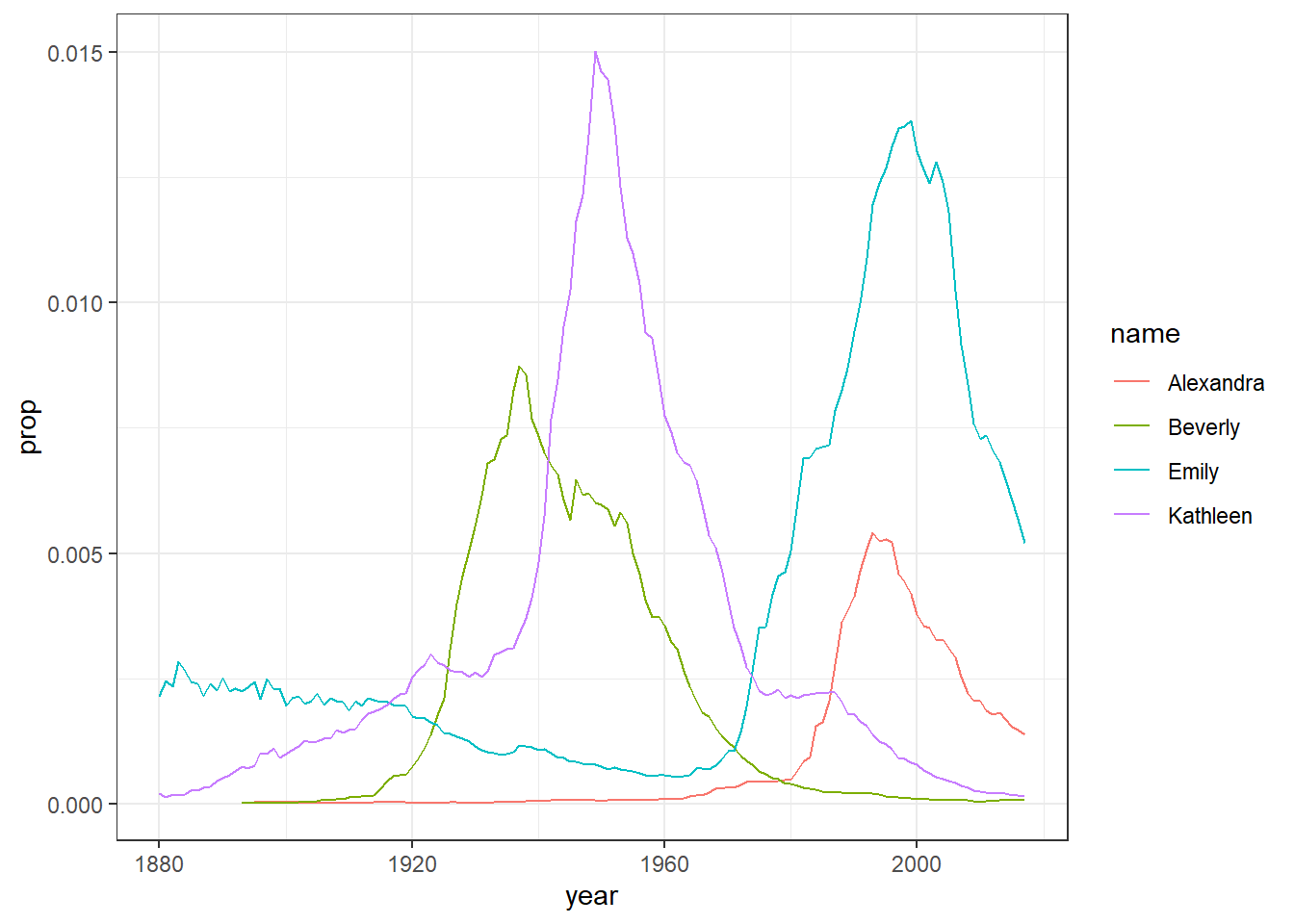
Figure 5.1: Proportion of four baby names from 1880 to 2014
- Change the names to your own examples and see how the plot changes. You can also change the sex from "F" to "M". Post the photos of your new plots on the Teams Data Skills channel.
- Because in most countries assigned sex at birth is binary, there is no data on intersex, trans or non-binary names. In lieu of that, here's the Wikipedia page about gender-neutral names and naming laws around the world which will hopefully make you question why on earth we ascribe someone's entire gender identity to a bunch of sounds and letters we use to label them.
This is more complicated than you might first imagine so only read on if you're feeling confident. If you remove the filter for sex when creating dat and then run the plot code again, it will make a very messy looking plot (try it). This is because for most names there will be two data points because although the numbers might be small for gendered names, there is usually always at least one baby of the non-dominant name gender that has been assigned that name.
You can get around this by adding an additional line of code that produces separate plots by sex. The scale argument tells R that it can use different scales on the y-axis for each plot - when there's a large difference between the two scales this is helpful to allow you to see the data in both sets (run this code and then remove the scales argument and run it again to see the difference) although it does run the risk of people misinterpreting the data if the difference between the scales isn't made clear.
dat2 <- babynames %>%
  filter(name %in% c("Emily","Kathleen","Alexandra","Beverly"))

ggplot(data = dat2,aes(x = year,y = prop, colour=name))+
  geom_line() +
  facet_wrap(~sex, scales = "free_y", nrow = 2)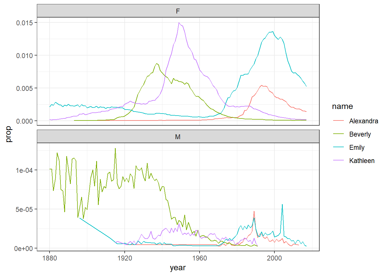
Figure 5.2: Plots by sex with different scales
On the other hand, if the scales for your two groups are fairly similar, it's better to keep the same scales to aid comparison. This time we will filter the dataset for gender neutral names where it might make more sense to have them on the same scale - again try it with and without the scales argument to see what happens
dat3 <- babynames %>%
  filter(name %in% c("Sam","Alex","Jordan","Drew"))

ggplot(data = dat3,aes(x = year,y = prop, colour=name))+
  geom_line() +
  facet_wrap(~sex, nrow = 2)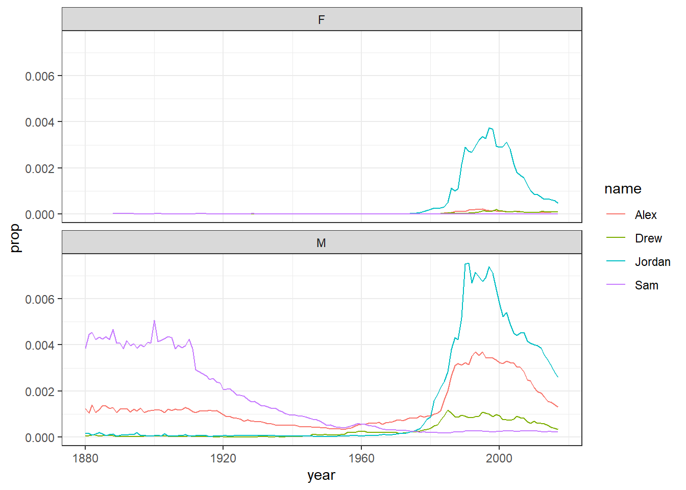
Figure 5.3: Plots by sex with the same scale
5.7 Activity 4: Selecting variables of interest
There are two numeric measurements of name popularity, prop (the proportion of all babies with each name) is probably more useful than n (total number of babies with that name), because it takes into account that different numbers of babies are born in different years.
Just like in Loading Data, if we wanted to create a dataset that only includes certain variables, we can use the select() function from the dplyr package. Run the below code to only select the columns year, sex, name and prop.
select(.data = babynames, # the object you want to select variables from
       year, sex, name, prop) # the variables you want to select
If you get an error message when using select that says
unused argument it means that it is trying to use the wrong
version of the select function. There are two solutions to this, first,
save you work and then restart the R session (click session -restart R)
and then run all your code above again from the start, or replace
select with dplyr::select which tells R
exactly which version of the select function to use. We'd recommend
restarting the session because this will get you in the habit and it's a
useful thing to try for a range of problems
Alternatively, you can also tell R which variables you don't want, in this case, rather than telling R to select year, sex, name and prop, we can simply tell it to drop the column n using the minus sign - before the variable name.
select(.data = babynames, -n)Note that select() does not change the original tibble, but makes a new tibble with the specified columns. If you don't save this new tibble to an object, it won't be saved. If you want to keep this new dataset, create a new object. When you run this code, you will see your new tibble appear in the environment pane.
new_dat <- select(.data = babynames, -n)5.8 Activity 5: Arranging the data
The function arrange() will sort the rows in the table according to the columns you supply. Try running the following code:
arrange(.data = babynames, # the data you want to sort
        name) # the variable you want to sort by
The data are now sorted in ascending alphabetical order by name. The default is to sort in ascending order. If you want it descending, wrap the name of the variable in the desc() function. For instance, to sort by year in descending order, run the following code:
You can also sort by more than one column. What do you think the following code will do?
5.9 Activity 6: Using filter to select observations
We have previously used select() to select certain variables or columns, however, frequently you will also want to select only certain observations or rows, for example, only babies born after 1999, or only babies named "Mary". You do this using the verb filter(). The filter() function is a bit more involved than the other verbs, and requires more detailed explanation, but this is because it is also extremely powerful.
Here is an example of filter, can you guess what it will do?
filter(.data = babynames, year > 2000)The first part of the code tells the function to use the object babynames. The second argument, year > 2000, is what is known as a Boolean expression: an expression whose evaluation results in a value of TRUE or FALSE. What filter() does is include any observations (rows) for which the expression evaluates to TRUE, and exclude any for which it evaluates to FALSE. So in effect, behind the scenes, filter() goes through the entire set of 1.8 million observations, row by row, checking the value of year for each row, keeping it if the value is greater than 2000, and rejecting it if it is less than 2000. To see how a boolean expression works, consider the code below:
years <- 1996:2005
years
years > 2000
## [1] 1996 1997 1998 1999 2000 2001 2002 2003 2004 2005
## [1] FALSE FALSE FALSE FALSE FALSE TRUE TRUE TRUE TRUE TRUEYou can see that the expression years > 2000 returns a logical vector (a vector of TRUE and FALSE values), where each element represents whether the expression is true or false for that element. For the first five elements (1996 to 2000) it is false, and for the last five elements (2001 to 2005) it is true.
Here are the most commonly used Boolean expressions.
| Operator | Name | is TRUE if and only if |
|---|---|---|
| A < B | less than | A is less than B |
| A <= B | less than or equal | A is less than or equal to B |
| A > B | greater than | A is greater than B |
| A >= B | greater than or equal | A is greater than or equal to B |
| A == B | equivalence | A exactly equals B |
| A != B | not equal | A does not exactly equal B |
| A %in% B | in | A is an element of vector B |
If you want only those observations for a specific name (e.g., Mary), you use the equivalence operator ==. Note that you use double equal signs, not a single equal sign.
filter(babynames, name == "Mary")If you wanted all the names except Mary, you use the 'not equals' operator:
filter(babynames, name!="Mary") And if you wanted names from a defined set - e.g., names of British queens - you can use %in%:
This gives you data for the names in the vector on the right hand side of %in%. You can always invert an expression to get its opposite. So, for instance, if you instead wanted to get rid of all Marys, Elizabeths, and Victorias you would use the following:
You can include as many expressions as you like as additional arguments to filter() and it will only pull out the rows for which all of the expressions for that row evaluate to TRUE. For instance, filter(babynames, year > 2000, prop > .01) will pull out only those observations beyond the year 2000 that represent greater than 1% of the names for a given sex; any observation where either expression is false will be excluded. This ability to string together criteria makes filter() a very powerful member of the Wickham Six.
Remember that this section exists. It will contain a lot of the answers to problems you face when wrangling data!
5.10 Activity 7: Creating new variables
Sometimes we need to create a new variable that doesn’t exist in our dataset. For instance, we might want to figure out what decade a particular year belongs to. To create new variables, we use the function mutate(). Note that if you want to save this new column, you need to save it to an object. Here, you are mutating a new column and attaching it to the new_dat object you created in Activity 4.
new_dat <- mutate(.data = babynames, # the tibble you want to add a column to
                  decade = floor(year/10) *10) # new column name = what you want it to contain
head(new_dat)| year | sex | name | n | prop | decade |
|---|---|---|---|---|---|
| 1880 | F | Mary | 7065 | 0.0723836 | 1880 |
| 1880 | F | Anna | 2604 | 0.0266790 | 1880 |
| 1880 | F | Emma | 2003 | 0.0205215 | 1880 |
| 1880 | F | Elizabeth | 1939 | 0.0198658 | 1880 |
| 1880 | F | Minnie | 1746 | 0.0178884 | 1880 |
| 1880 | F | Margaret | 1578 | 0.0161672 | 1880 |
In this case, you are creating a new column decade which has the decade each year appears in. This is calculated using the command decade = floor(year/10)*10.
5.11 Activity 8: Grouping and summarising
Most quantitative analyses will require you to summarise your data somehow, for example, by calculating the mean, median or a sum total of your data. You can perform all of these operations using the function summarise().
First, let's use the object dat that just has the data for the four girls names, Alexandra, Beverly, Emily, and Kathleen. To start off, we're simply going to calculate the total number of babies across all years that were given one of these four names.
It's useful to get in the habit of translating your code into full sentences to make it easier to figure out what's happening. You can read the below code as "run the function summarise using the data in the object dat to create a new variable named total that is the result of adding up all the numbers in the column n".
| total |
|---|
| 2161374 |
summarise() becomes even more powerful when combined with the final dplyr function, group_by(). Quite often, you will want to produce your summary statistics broken down by groups, for examples, the scores of participants in different conditions, or the reading time for native and non-native speakers.
There are two ways you can use group_by(). First, you can create a new, grouped object.
group_dat <- group_by(.data = dat, # the data you want to group
                      name) # the variable you want to group by
If you look at this object in the viewer, it won't look any different to the original dat, however, the underlying structure has changed. Let's run the above summarise code again, but now using the grouped data.
| name | total |
|---|---|
| Alexandra | 231364 |
| Beverly | 376914 |
| Emily | 841491 |
| Kathleen | 711605 |
summarise() has performed exactly the same operation as before - adding up the total number in the column n - but this time it has done is separately for each group, which in this case was the variable name.
You can request multiple summary calculations to be performed in the same function. For example, the following code calculates the mean and median number of babies given each name every year.
| name | mean_year | median_year |
|---|---|---|
| Alexandra | 1977.470 | 192.0 |
| Beverly | 3089.459 | 709.5 |
| Emily | 6097.761 | 1391.5 |
| Kathleen | 5156.558 | 3098.0 |
You can also add multiple grouping variables. For example, the following code groups new_dat by sex and decade and then calculates the summary statistics to give us the mean and median number of male and female babies in each decade.
group_new_dat <- group_by(new_dat, sex, decade)
summarise(group_new_dat,
          mean_year = mean(n),
          median_year = median(n))
## `summarise()` has grouped output by 'sex'. You can override using the `.groups`
## argument.| sex | decade | mean_year | median_year |
|---|---|---|---|
| F | 1880 | 110.57017 | 13 |
| F | 1890 | 128.18406 | 13 |
| F | 1900 | 131.32904 | 12 |
| F | 1910 | 187.06284 | 12 |
| F | 1920 | 210.54574 | 12 |
| F | 1930 | 214.19867 | 12 |
| F | 1940 | 262.20824 | 12 |
| F | 1950 | 288.47692 | 13 |
| F | 1960 | 234.71960 | 12 |
| F | 1970 | 147.20851 | 11 |
| F | 1980 | 134.25355 | 11 |
| F | 1990 | 113.07160 | 11 |
| F | 2000 | 96.45799 | 11 |
| F | 2010 | 91.69925 | 11 |
| M | 1880 | 100.76497 | 12 |
| M | 1890 | 93.59019 | 12 |
| M | 1900 | 94.38963 | 12 |
| M | 1910 | 180.83854 | 12 |
| M | 1920 | 226.78161 | 13 |
| M | 1930 | 253.28957 | 13 |
| M | 1940 | 368.40859 | 14 |
| M | 1950 | 460.86555 | 14 |
| M | 1960 | 415.51792 | 13 |
| M | 1970 | 265.55153 | 12 |
| M | 1980 | 236.98189 | 11 |
| M | 1990 | 187.35187 | 11 |
| M | 2000 | 149.06677 | 11 |
| M | 2010 | 133.67495 | 11 |
If you get what looks like an error that says
summarise() ungrouping output (override with .groups argument)don't
worry, this isn't an error it's just R telling you what it's done. This
message was included in a very recent update to the
tidyverse which is why it doesn't appear on some of the
walkthrough vidoes.
5.12 Activity 9: Pipes
The final activity for this chapter essentially repeats what we've already covered but in a slightly different way. In the previous activities, you created new objects with new variables or groupings and then you called summarise() on those new objects in separate lines of code. As a result, you had multiple objects in your environment pane and you need to make sure that you keep track of the different names.
Instead, you can use pipes. Pipes are written as %>%and they should be read as "and then". Pipes allow you to string together 'sentences' of code into 'paragraphs' so that you don't need to create intermediary objects. Again, it is easier to show than tell.
The below code does exactly the same as all the code we wrote above but it only creates one object.
pipe_summary <- mutate(babynames, decade = floor(year/10) *10) %>%
  filter(name %in% c("Emily","Kathleen","Alexandra","Beverly"), sex=="F") %>%
  group_by(name, decade) %>%
  summarise(mean_decade = mean(n))
The reason that this function is called a pipe is because it 'pipes' the data through to the next function. When you wrote the code previously, the first argument of each function was the dataset you wanted to work on. When you use pipes it will automatically take the data from the previous line of code so you don't need to specify it again.
When learning to code it can be a useful practice to read your code 'out loud' in full sentences to help you understand what it is doing. You can read the code above as "create a new variable called decade AND THEN only keep the names Emily, Kathleen, Alexandra and Beverly that belong to female babies AND THEN group the dataset by name and decade AND THEN calculate the mean number of babies with each name per decade." Try doing this each time you write a new bit of code.
Some people find pipes a bit tricky to understand from a conceptual point of view, however, it's well worth learning to use them as when your code starts getting longer they are much more efficient and mean you have to write less code which is always a good thing!
5.13 Finished!
That was a long chapter but remember, you don't need to memorise all of this code. You just need to know where to look for help. Finally, if you're working from the R server, we'd recommend that you download a copy of the changes you've made to stub-wrangling-1 so that you have a backup.