6 1B: Lab 1

6.1 Pre-class activities

6.1.1 Welcome back!

Welcome back to Psych 1B! This semester we’re going to build on the data skills you developed in the first semester by adding in a couple of new data wrangling functions, running probability simulations in preparation for statistics in level 2, and analysing your own data for the group project.

It would be nice to always get data formatted in the way that you want it, but one of the challenges as a scientist is dealing with Other People’s Data. People often structure data in ways that is convenient for data entry, but not very convenient for data analysis, and so, much effort must be expended ’wrangling’ data into shape before you can do more interesting things with it. Additionally, performing analyses often requires pulling together data obtained from different sources: you have done this in semester 1 by combining the participant information with the depression and happiness data. In this semester, we are going to give you some tips on how to structure data, and introduce strategies for transforming and combining data from different sources.

6.1.2 Autism-quotient data

For Psych 1B we’re going to use a different dataset for our exercises based upon data that was collected using SurveyMonkey but that has has simulated variables added for the purposes of these exercises (gender was missing, so we have added this in). For this research project, participants completed the short 10-item version of the Autism-Spectrum Quotient (AQ) (Baron-Cohen, Wheelwright, Skinner, Martin, & Clubley, 2001), which is designed to measure autistic traits in adults. The items for the quetionnaire are shown below.

Table 1: The ten items on the AQ-10.

Q_No	Question
Q 1	I often notice small sounds when others do not.
Q 2	I usually concentrate more on the whole picture, rather than small details.
Q 3	I find it easy to do more than one thing at once.
Q 4	If there is an interruption, I can switch back to what I was doing very quickly.
Q 5	I find it easy to read between the lines when someone is talking to me.
Q 6	I know how to tell if someone listening to me is getting bored.
Q 7	When I’m reading a story, I find it difficult to work out the characters’ intentions.
Q 8	I like to collect information about categories of things.
Q 9	I find it easy to work out what someone is thinking or feeling just by looking at their face.
Q 10	I find it difficult to work out people’s intentions.

Responses to each item were measured on a four-point scale: Definitely Disagree, Slightly Disagree, Slightly Agree, Definitely Agree. One of the issues with conducting research using surveys is that if we don’t design them carefully, our data may be affected by response bias. One type of response bias is acquiescence bias, which is the finding that people have a tendancy to agree with all statements. To try and minimise the impact of this, many questionnaires will reverse-code some of the questions so that a positive response means agreeing with one question but disagreeing with another.

Read through the questions. Type the number of one of the items where you think agreeing with the item would mean the participant displayed autistic traits
Now type the number of one of the items where you think disagreeing with the item would mean the participant displayed autistic traits

For those items where agreeing with the item means a higher autistic quotient (AQ) score, participants recieve a score of 1 if they answer “Slightly agree” or “Agree”. This is called forward scoring. For those items where disagreeing with the item means a higher AQ score, participants recieve a score of 1 if they answer “Slightly disagree” or “Disagree”. This is know as reverse coding.

The AQ score for each participant is the total score (i.e., the sum) of all 10 questions. The higher the AQ score, the more ’autistic traits’ they are assumed to exhibit and it is this score we are interested in.

6.1.3 Activity 1: Download the data

Create a new folder for your Psych 1B data skills work. Do not call the folder “R” as this can cause R to have an existential crisis that it’s saving into itself.
Download the Psych 1B zip file, extract the files, and then move the three csv files to the folder you created above.

6.1.4 Activity 2: Open a new Markdown document

In Psych 1A, we provided the Markdown documents for you in the form of stub files. From this point on, you’re going to create and save your own.

Open R Studio and set the working directory to your Psych 1B folder. If this has worked, you should see the csv files you just downloaded in the file pane in the bottom right of R Studio.
To open a new R Markdown document click the ‘new item’ icon and then click ‘R Markdown’. You will be prompted to give it a title, call it “Lab 1 pre-class”. Also, change the author name to your GUID as this will be good practice for the homework. Keep the output format as HTML.
Once you’ve opened a new document be sure to save it by clicking File -> Save as. Name this file “Lab 1 pre-class”. If you’ve set the working directory correctly, you should now see this file appear in your file viewer pane.

Figure 6.1: Opening a new R Markdown document

6.1.5 Activity 3: Create a new code chunk

When you first open a new R Markdown document you will see a bunch of default welcome text. Do the following steps:

Delete everything below line 7
On line 8 type “Activity 3”
Click Insert -> R

Figure 6.2: New R chunk

You should create a new code chunk for each activity or each analysis step and make sure there is a description of what the code is doing. This will make it easier to read your Markdown and find where any errors in the code are. Do not put all of your code in one big chunk.

6.1.6 Activity 4: Load in the data

Type and run the code that loads the tidyverse package.
Use read_csv() to load in the data. you should create three objects responses, scoring and qformats that contain the respective data. If you need help remembering how to load in data files, check Psych 1A, Lab 2 Activity 4.

The solutions are at the bottom if you need them. However, remember what you learned about memory and learning in Psych 1A, you’ll learn more if you try and retrieve the code from memory. There were a couple of comments in the 1A EvaSys that said some of you felt like you were just copying and pasting - this can only be true if you choose to copy and paste.

6.1.7 Activity 5: Look at the data

View each of the three datasets by clicking on their name in the environment.
Check each object by using summary(), e.g., summary(qformats).
responses contains the actual data from the survey. There is a participant Id column and then the rest of the columns contain the responses associated with that participant for each of the 10 questions (Q1, Q2, Q3, …, Q10).
scoring contains the scoring information that we described above, that is, whether a question should be given a score of 1 or 0 for forward and reverse coded items for each possible response.
qformats contains a list of whether each question is forward or reverse coded.

6.1.8 Thinking through the problem

In order to get a total AQ score for each participant, we need to combine the information from all three files, that is, we need to know the participants response and then how to score it. We technically could score the data by hand. However, there are 66 participants in this dataset with each participant providing 10 responses. This means we would have to manually tidy up 660 responses.

Not only would this be a horribly mind-numbing task, it is also one in which you would be prone to make errors. Even if you were 99% accurate, you would still get about 7 of the scores wrong. Worst of all, this approach does not scale beyond small datasets. When you analyse the data from your group project, there will likely be thousands of participants and you don’t have time to do these by hand!

Pause here and think about how you might calculate AQ scores for each participant. What are the necessary steps?

Let’s imagine we are doing the task by hand so that we understand the logic. Once that logic is clear, we’ll go through it again and show you how to write the script to make it happen.

Let’s take stock of what we know. First, we know that there are two question formats, and that questions Q1, Q7, Q8, and Q10 are scored according to format F and questions Q2, Q3, Q4, Q5, Q6, and Q9 are scored according to format R. This is the information that is currently stored in qformats:

Question	QFormat
Q 1	F
Q 2	R
Q 3	R
Q 4	R
Q 5	R
Q 6	R
Q 7	F
Q 8	F
Q 9	R
Q 10	F

We also know that for format F, we award a point for agree, zero for disagree. For format R, a point for disagree, zero for agree. This is the information that is currently stored in scoring:

QFormat	Response	Score
F	Definitely Agree	1
F	Slightly Agree	1
F	Slightly Disagree	0
F	Definitely Disagree	0
R	Definitely Agree	0
R	Slightly Agree	0
R	Slightly Disagree	1
R	Definitely Disagree	1

Finally, we would need to look at the responses from each participant and then give them the correct score for the format of the question. Let’s walk through the example with the first participant. For this participant (Id = 16), we have the following responses:

Question	Participant 16 Response
Q 1	Slightly Disagree
Q 2	Definitely Agree
Q 3	Slightly Disagree
Q 4	Definitely Disagree
Q 5	Slightly Agree
Q 6	Slightly Agree
Q 7	Slightly Agree
Q 8	Definitely Disagree
Q 9	Slightly Agree
Q 10	Slightly Agree

Note that we have re-formatted the responses so that each response is in a separate row, rather than having all of the responses in a single row, as they are in responses. We have reshaped the data from its original wide format to long format. This format is called long because instead of having just one row for each participant, we now have one row for each data point and so 10 rows for each participant.

While this format makes it less easy to read the whole dataset in with a single glance, it actually ends up being much easier to deal with, because ’Question’ is a now a single variable whose levels are Q1, Q2, …, Q10, and ’Response’ is also now a single variable. Most functions that you will be working with in R will expect your data to be in long rather than wide format.

Let’s now look up the format for each question:

Question	Participant 16 Response	QFormat
Q 1	Slightly Disagree	F
Q 2	Definitely Agree	R
Q 3	Slightly Disagree	R
Q 4	Definitely Disagree	R
Q 5	Slightly Agree	R
Q 6	Slightly Agree	R
Q 7	Slightly Agree	F
Q 8	Definitely Disagree	F
Q 9	Slightly Agree	R
Q 10	Slightly Agree	F

And now that we have the format and the response, we can look up the scores:

Question	Participant 16 Response	QFormat	Score
Q 1	Slightly Disagree	F	0
Q 2	Definitely Agree	R	0
Q 3	Slightly Disagree	R	1
Q 4	Definitely Disagree	R	1
Q 5	Slightly Agree	R	0
Q 6	Slightly Agree	R	0
Q 7	Slightly Agree	F	1
Q 8	Definitely Disagree	F	0
Q 9	Slightly Agree	R	0
Q 10	Slightly Agree	F	1

Then we just add up the scores, which yields an AQ score of 4 for participant 16. We would then repeat this logic for the remaining 65 participants. Anyone fancy doing this for a big data set?!

Due to the large margin for error in carrying out this task by hand, it’s important to learn how to make the computer do the dirty work. The computer won’t make mistakes and will free up your mind to focus on the bigger issues in your research.

6.1.9 Activity 5: Recap

Finally, let’s refresh your memory of some of the important tidyverse functions before the labs begin.

What function would you use to keep just the columns Q1 and Q2 in responses?
What function would you use to keep just the data from participant 16 in reponses?
What function would you use to add up the total score for participant 16?
What function would you use to join together qformats and scoring?

6.1.10 Activity 6: Reading and revision

The final part of the pre-class involves some reading - head to the Lab 1 section of the 1B practical page on Moodle to get the materials.

If you struggled with R last semester, please make sure that you revise the material from [1A - Lab 1])https://psyteachr.github.io/ug1-practical/a-lab-1.html#homework in particular as it explains a lot of the basics of R and it may help you to revisit this material. There will be an R catch-up session held by our of our GTAs Rebecca Lai on Wednesday 15th January Boyd Orr 603, 12:00 - 15:00.

6.1.11 Activity solutions

6.1.11.1 Activity 4

library(tidyverse)
scoring <- read_csv ("scoring.csv")
responses <- read_csv("responses.csv")
qformats <- read_csv("qformats.csv")

6.2 In-class activities

Let’s continue what we started in the pre-class activities by hand but now using R to calculate a score for each participant.

6.2.1 Activity 1: Load in the data

Open a new R markdown document, name it “Lab 1 in-class” and save it in your Psych 1B folder.
Set the working directory to your Psych 1B folder.
Type and run the code that loads the tidyverse package.
Use read_csv() to load in the data. you should create three objects responses, scoring and qformats that contain the respective data.

6.2.2 Activity 2: `pivot_longer()`

The first step is to transform our data from wide format to long format. To do this, we will use the function pivot_longer(). pivot_longer() takes multiple columns and collapses them so that each unique variable has it’s own column and has four main arguments:

data is the name of the object you want to transform
names_to is the name of the new column that you will create that will contain the names of the original wide format columns
values_to is the name of the column that will contain the existing values.
cols are the original columns you want to collapse.

These functions can seem a bit abstract and it is better to show than tell. Run the below code in a new code chunk and then compare how rlong looks compared to responses and see if you can figure out what effect each argument had.

rlong <- pivot_longer(data = responses, 
                      names_to = "Question",  
                      values_to = "Response",
                      cols = Q1:Q10)

You have now created a tibble with 660 observations and 3 variables; 10 observations per 66 participants and 3 variables. Let’s recreate the example from the pre-class only use one participant. We can do that by using filter() which you used last semester and creating a new tibble called rlong_16.

6.2.3 Activity 3: `filter()`

Pause here and test your knowledge

What does filter() do?

Create a new object called rlong_16
Use filter() to keep only the data from participant Id 16.

Every year, the biggest problem with these exercises is typos caused by not paying attention to the exact spelling and capitalisation. Remember, Question is not the same as question, Response is not the same as response, and Id is not the same as ID.

6.2.4 Activity 4: `inner_join()`

The next step is to match each question with its format (F or R) that is stored in qformats. That is, we need to join together the two objects using inner_join() like we did in Psych 1A.

Create a new object called rlong_16_join that uses inner_join() to join together rlong_16 and qformatsby their common column.
If you get the error Error: by can't contain join column XXXX which is missing from LHS it means that you have made a typo. Check the exact spelling and capitalisation of the variable names.

What inner_join() does is match up rows in the two tables where both tables have the same value for the field named in the third argument, “Question”; it then combines the columns from the two tables, copying rows where necessary.

To state it more simply, what it does, in effect, is the following: For each row in rlong, it checks the value of the column Question, and looks for rows with the same value in qformats, and then essentially combines all of the other columns in the two tables for these matching rows. If there are unmatching values, the rows get dropped. The inner_join() is one of the most useful and time-saving operations in data wrangling so keep ptracticing as it will keep reappearing time after time.

6.2.5 Activity 5: Another `inner_join()`

Now that we have matched up each question with its corresponding format, we can now “look up” the corresponding scores in the scoring table based on the format and the response. This means we have to use inner_join() once again to join rlong_16_join with scoring**

Create a new object named scores_16 than joins together rlong_16_join with scoring.
Be careful to tell R all of the columns the two objects have in common. Remember that when you need to specify multiple variables you will need to use the syntax by = c("var1", "var2).

6.2.6 Activity 6: Calculating the AQ score

Now you need to calculate the total AQ score for participant 16.

Create a new object called AQ_16. Use summarise() and sum()to add up the numbers in the column Score from scores_16 and call the result of this calculation AQ_score.
This is quite a difficult task to do from memory but try it anyway - if you get anywhere near the right solution you’re doing extremely well!

6.2.7 Activity 7: Calculating all scores

Next we’re going to do the same thing but for all participants. The first two steps are the same but we just use the full data rlong rather than the filtered dataset.

Run the below code in a new code chunk.

rlong_join <- inner_join(rlong, qformats, "Question")
scores <- inner_join(rlong_join, scoring, c("QFormat", "Response"))

The final part of calculating the scores requires an extra step because now we don’t just want to calculate one score, we want to calculate a score for each participant which means that we need to use group_by() to group by Id. We’re not going to use it in this lab but we also want our object to show us the participant’s gender so we will also add gender to the grouping. If you want to refresh your memory about how group_by() works, revise Psych 1A Lab 3 Activity 8.

scores_grouped <- group_by(scores, Id, gender)
AQ_all <- summarise(scores_grouped, total_score = sum(Score))

6.2.8 Activity 8: Visualisation

Finally, use ggplot() and geom_histogram() to make a histogram of all the total AQ scores. Try and make it look pretty by changing the axis labels and the theme. You can check the solution code to see how the below example was made, but you can make yours look different.

Hint 1: ggplot(data, aes(x)) + geom_histogram()
Hint 2: Add binwidth = 1 to geom_histogram() to change the width of the bars.

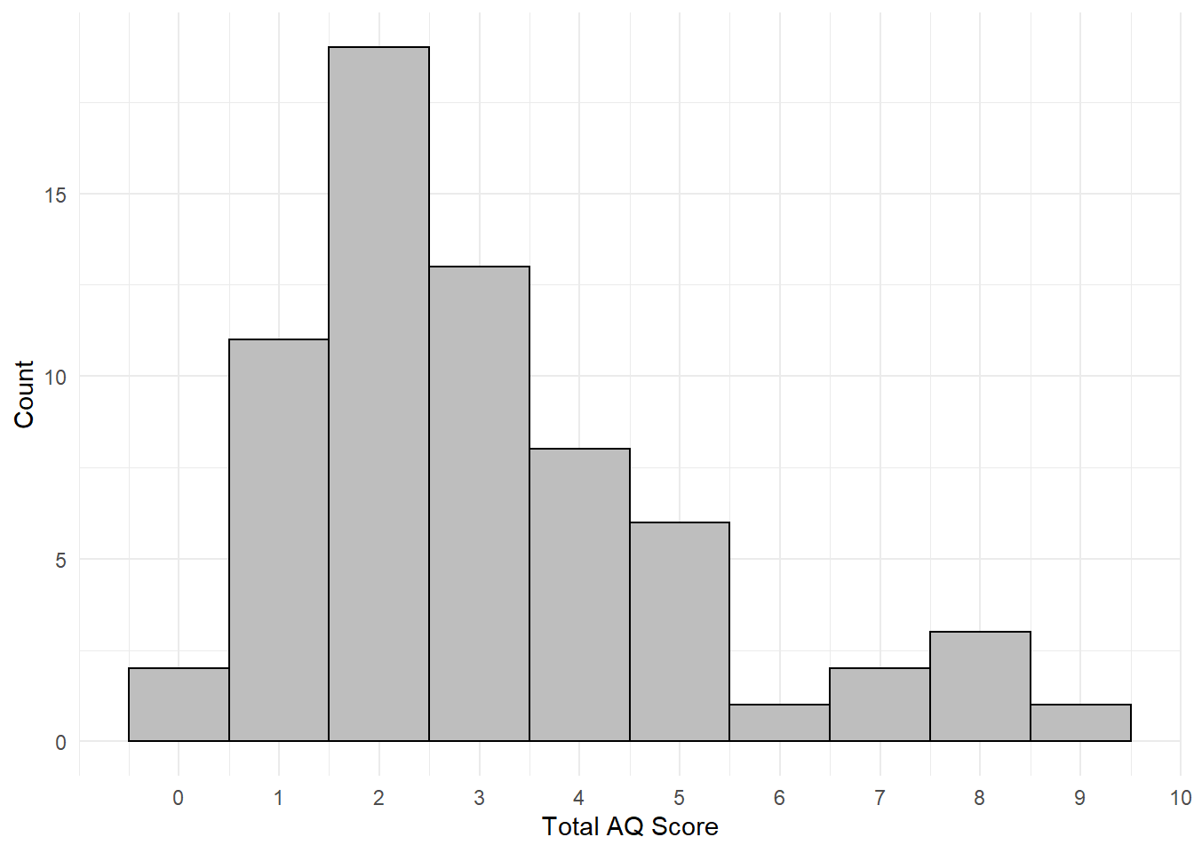
Figure 6.3: Histogram of total AQ scores

6.2.9 Activity solutions

6.2.9.1 Activity 1

library(tidyverse)
scoring <- read_csv ("scoring.csv")
responses <- read_csv("responses.csv")
qformats <- read_csv("qformats.csv")

6.2.9.2 Activity 3

rlong_16 <- filter(rlong, Id == 16)

6.2.9.3 Activity 4

rlong_16_join <- inner_join(rlong_16, qformats, "Question")

6.2.9.4 Activity 5

scores_16 <- inner_join(rlong_16_join, scoring, c("QFormat", "Response"))

6.2.9.5 Activity 6

AQ_16 <- summarise(scores_16, AQ_score = sum(Score))

6.2.9.6 Activity 8

ggplot(AQ_all, aes(x = total_score)) +
  geom_histogram(binwidth = 1, colour = "black", fill = "grey") +
  theme_minimal()+
  scale_x_continuous(name = "Total AQ Score", breaks = c(0,1,2,3,4,5,6,7,8,9,10)) +
  scale_y_continuous(name = "Count")