This chapter closes the coding section because writing code with AI represents the highest-risk, highest-reward use case. By this point, you should be able to judge when AI suggestions are useful scaffolds and when they are dangerous shortcuts.
The best AI platform for writing code is arguably Github Copilot (or Super Clippy as my programmer friends like to call it) and there are also specialised packages that you integrate LLMs into RStudio. However, unless coding is the main part of your job, most people are likely to use AI through a generic platform so we’ll stick with regular Copilot.
If you have access to LinkedIn Learning (which you do if you are a UofG student or staff), I’d also highly recommend the short course Pair Programming with AI by Morten Rand-Hendriksen. It only takes 1.5 hours to work through and he covers using both Github Copilot and ChatGPT and has a nicely critical view of AI.
If you’ve worked through this entire book then hopefully what you’ve learned is that AI is very useful but you should also have a healthy mistrust of anything it produces which is why this chapter is the last in the coding section.
The number 1 rule to keep in mind when using AI to write code is that the platforms we’re using are not intelligent. They are not thinking. They are not reasoning. They are not telling the truth or lying to you. They don’t have gaps in their knowledge because they have no knowledge. They are digital parrots on cocaine.
The dataset is massive so as our first task, we want to write code that narrows it down and creates three different objects.
First, we want to create an object named demo that has the demographic information, age and gender. Age data has transformed into categories (e.g., 18-21) for anonymisation purposes. The option ‘Implausible’ describes values that were 99 or higher or 17 or lower.
Second, we want an object named STARS which will represent each participant’s score on the Statistics Anxiety Rating Scale (STARS; Cruise et al., 1985). Each item describes a situation involving statistics such as “Doing an examination in a statistics course” (test and class anxiety), “Interpreting the meaning of a table in a journal article” (interpretation anxiety), or “Going to ask my statistics teacher for individual help with material I am having difficulty understanding” (fear of asking for help).
Third, we want an object named, IUS which will represent each participant’s score on the Intolerance of Uncertainty Scale – Short Form (IUS-SF; Carleton et al., 2007). The scale contains 2 subscales, Prospective Anxiety and Inhibitory Anxiety, each with 6 items. The Prospective Anxiety subscale includes statements such as, “The smallest doubt can stop me from acting”. The Inhibitory Anxiety subscale includes statements such as, “It frustrates me not having all the information I need”.
For the two scales, we need to pivot it to long-form and then calculate the mean score for each participant.
We would need this information if we wanted to try and answer questions like:
What is the demographic make-up of the sample in terms of age and gender?
How is statistics anxiety and intolerance of uncertainty related?
Do men and women differ in their level of statistics anxiety?
But we’ll start with the wrangling and see how far we get.
Activity 1
First, download the dataset from the Open Science Framework. Create a new Quarto or Rmd document and ensure the dataset is in the same folder, as this document, and then run the below code in a new code chunk. This will load in the data and then it will create the three objects using the code I have written and the approach I have taken so that we can compare with how Copilot gets on.
This is such a large dataset that we will just select the columns we need, but bear in mind I have already made the task easier for the AI by doing so.
Warning: package 'tidyverse' was built under R version 4.3.2
Warning: package 'tidyr' was built under R version 4.3.3
Warning: package 'readr' was built under R version 4.3.3
Warning: package 'dplyr' was built under R version 4.3.3
Warning: package 'stringr' was built under R version 4.3.3
Warning: package 'lubridate' was built under R version 4.3.3
library(tidyverse)# load in the data and just select the columns we will needdat <-read_csv("smarvus_complete_050524.csv") |>select(unique_id, age, gender, Q7.1_1:Q7.1_24, Q14.1_1:Q14.1_12)# pull out demographic datademo <- dat %>%select(unique_id, age, gender) |>drop_na()# create statistics anxiety scaleSTARS <- dat %>%select(unique_id, Q7.1_1:Q7.1_24) %>%# select the STARS columnsfilter(Q7.1_24 ==1) %>%# remove those who failed the attention checkselect(-Q7.1_24) %>%# remove the attention check columnpivot_longer(cols = Q7.1_1:Q7.1_23, names_to ="item", values_to ="score") %>%# transform to long-formgroup_by(unique_id) %>%# group by participantsummarise(stars_score =mean(score)) %>%# calculate mean STARS score for each pptungroup() %>%# ungroup so it doesn't mess things up laterdrop_na() # get rid of NAs so they don't cause us havoc# Intolerance of Uncertainty.IUS <- dat %>%select(unique_id, Q14.1_1:Q14.1_12) %>%# select the BNFE columnspivot_longer(cols = Q14.1_1:Q14.1_12, names_to ="item", values_to ="score") %>%# transform to long-formgroup_by(unique_id) %>%# group by participantsummarise(ius_score =mean(score)) %>%# calculate mean IUS-SF score for each pptungroup() %>%# ungroup so it doesn't mess things up laterdrop_na() # get rid of NAs so they don't cause us havoc# join it all togetherdat_joined <-left_join(demo, IUS) |>left_join(STARS)
6.2 Prompting
Now we want to do some set-up to prompt the AI to help us write code that works and does what we want.
Activity 2
In Copilot, enter the following prompt:
You are an expert R programmer. Help me write tidyverse-first code. Before writing code, ask any clarifying questions needed about data, objectives, constraints, and outputs.When you do write code:
Use tidyverse idioms (|>, dplyr, ggplot2, tibble), no deprecated functions. Comment clearly and explain non-obvious choices (e.g., NA handling, binning, model specs). Be safe and reproducible: no setwd(), no absolute paths, no silent package installs; show any set.seed() if randomness is used. Handle missing data explicitly and avoid destructive transformations.
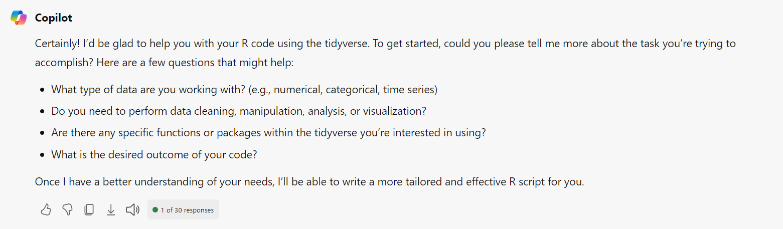
When you input this starting prompt, there’s a good chance you’ll get something like the following:
More info needed
6.3 Describing your dataset
As I may have mentioned once or twice in this book, there is no substitute for knowing your data. For the dataset provided here, your first step as an analyst would be to read the paper in full so that you understand how and what data was collected, the scales of measurement, and information about missing data etc.
In addition to this domain knowledge, you can also use information R provides about the dataset to help you.
summary() is useful because it provides a list of all variables with some descriptive statistics so that the AI has a sense of the type and range of data:
summary(dat)
  unique_id             age               gender              Q7.1_1
 Length:12570       Length:12570       Length:12570       Min.   :1.000
 Class :character   Class :character   Class :character   1st Qu.:2.000
 Mode  :character   Mode  :character   Mode  :character   Median :3.000
                                                          Mean   :3.229
                                                          3rd Qu.:4.000
                                                          Max.   :5.000
                                                          NA's   :457
     Q7.1_2          Q7.1_3          Q7.1_4          Q7.1_5
 Min.   :1.000   Min.   :1.000   Min.   :1.000   Min.   :1.000
 1st Qu.:2.000   1st Qu.:2.000   1st Qu.:2.000   1st Qu.:2.000
 Median :3.000   Median :3.000   Median :3.000   Median :3.000
 Mean   :2.696   Mean   :2.817   Mean   :2.858   Mean   :2.687
 3rd Qu.:4.000   3rd Qu.:4.000   3rd Qu.:4.000   3rd Qu.:4.000
 Max.   :5.000   Max.   :5.000   Max.   :5.000   Max.   :5.000
 NA's   :458     NA's   :453     NA's   :451     NA's   :457
     Q7.1_6          Q7.1_7          Q7.1_8          Q7.1_9        Q7.1_10
 Min.   :1.000   Min.   :1.000   Min.   :1.000   Min.   :1.00   Min.   :1.000
 1st Qu.:1.000   1st Qu.:2.000   1st Qu.:3.000   1st Qu.:1.00   1st Qu.:3.000
 Median :2.000   Median :3.000   Median :4.000   Median :2.00   Median :4.000
 Mean   :2.424   Mean   :3.167   Mean   :3.841   Mean   :2.03   Mean   :3.647
 3rd Qu.:3.000   3rd Qu.:4.000   3rd Qu.:5.000   3rd Qu.:3.00   3rd Qu.:5.000
 Max.   :5.000   Max.   :5.000   Max.   :5.000   Max.   :5.00   Max.   :5.000
 NA's   :467     NA's   :461     NA's   :454     NA's   :457    NA's   :459
    Q7.1_11         Q7.1_12         Q7.1_13         Q7.1_14
 Min.   :1.000   Min.   :1.000   Min.   :1.000   Min.   :1.000
 1st Qu.:2.000   1st Qu.:1.000   1st Qu.:2.000   1st Qu.:2.000
 Median :3.000   Median :2.000   Median :3.000   Median :3.000
 Mean   :2.698   Mean   :2.583   Mean   :3.374   Mean   :2.654
 3rd Qu.:4.000   3rd Qu.:4.000   3rd Qu.:4.000   3rd Qu.:4.000
 Max.   :5.000   Max.   :5.000   Max.   :5.000   Max.   :5.000
 NA's   :461     NA's   :454     NA's   :462     NA's   :459
    Q7.1_15         Q7.1_16         Q7.1_17         Q7.1_18
 Min.   :1.000   Min.   :1.000   Min.   :1.000   Min.   :1.000
 1st Qu.:3.000   1st Qu.:2.000   1st Qu.:1.000   1st Qu.:1.000
 Median :4.000   Median :3.000   Median :2.000   Median :2.000
 Mean   :3.607   Mean   :2.711   Mean   :2.362   Mean   :2.461
 3rd Qu.:5.000   3rd Qu.:4.000   3rd Qu.:3.000   3rd Qu.:3.000
 Max.   :5.000   Max.   :5.000   Max.   :5.000   Max.   :5.000
 NA's   :452     NA's   :463     NA's   :457     NA's   :460
    Q7.1_19         Q7.1_20         Q7.1_21         Q7.1_22
 Min.   :1.000   Min.   :1.000   Min.   :1.000   Min.   :1.000
 1st Qu.:2.000   1st Qu.:2.000   1st Qu.:1.000   1st Qu.:2.000
 Median :2.000   Median :3.000   Median :2.000   Median :3.000
 Mean   :2.612   Mean   :2.735   Mean   :2.576   Mean   :3.048
 3rd Qu.:4.000   3rd Qu.:4.000   3rd Qu.:4.000   3rd Qu.:4.000
 Max.   :5.000   Max.   :5.000   Max.   :5.000   Max.   :5.000
 NA's   :453     NA's   :458     NA's   :458     NA's   :463
    Q7.1_23         Q7.1_24         Q14.1_1         Q14.1_2
 Min.   :1.000   Min.   :1.000   Min.   :1.000   Min.   :1.000
 1st Qu.:1.000   1st Qu.:1.000   1st Qu.:2.000   1st Qu.:3.000
 Median :2.000   Median :1.000   Median :3.000   Median :4.000
 Mean   :2.314   Mean   :1.161   Mean   :2.927   Mean   :3.465
 3rd Qu.:3.000   3rd Qu.:1.000   3rd Qu.:4.000   3rd Qu.:4.000
 Max.   :5.000   Max.   :5.000   Max.   :5.000   Max.   :5.000
 NA's   :460     NA's   :1306    NA's   :1497    NA's   :1500
    Q14.1_3         Q14.1_4         Q14.1_5         Q14.1_6
 Min.   :1.000   Min.   :1.000   Min.   :1.000   Min.   :1.000
 1st Qu.:2.000   1st Qu.:2.000   1st Qu.:2.000   1st Qu.:1.000
 Median :3.000   Median :3.000   Median :3.000   Median :2.000
 Mean   :2.682   Mean   :2.974   Mean   :2.702   Mean   :2.527
 3rd Qu.:4.000   3rd Qu.:4.000   3rd Qu.:4.000   3rd Qu.:3.000
 Max.   :5.000   Max.   :5.000   Max.   :5.000   Max.   :5.000
 NA's   :1500    NA's   :1497    NA's   :1499    NA's   :1498
    Q14.1_7         Q14.1_8         Q14.1_9         Q14.1_10
 Min.   :1.000   Min.   :1.000   Min.   :1.000   Min.   :1.000
 1st Qu.:2.000   1st Qu.:2.000   1st Qu.:2.000   1st Qu.:2.000
 Median :3.000   Median :3.000   Median :3.000   Median :3.000
 Mean   :3.008   Mean   :3.168   Mean   :2.667   Mean   :2.676
 3rd Qu.:4.000   3rd Qu.:4.000   3rd Qu.:4.000   3rd Qu.:4.000
 Max.   :5.000   Max.   :5.000   Max.   :5.000   Max.   :5.000
 NA's   :1498    NA's   :1500    NA's   :1499    NA's   :1496
    Q14.1_11        Q14.1_12
 Min.   :1.000   Min.   :1.00
 1st Qu.:2.000   1st Qu.:2.00
 Median :3.000   Median :3.00
 Mean   :3.228   Mean   :2.64
 3rd Qu.:4.000   3rd Qu.:4.00
 Max.   :5.000   Max.   :5.00
 NA's   :1496    NA's   :1500
str() is also useful because it lists the variables, their data type, and the initial values for each variable. However, that means that you are giving it at least some of the raw data so you have to be very careful if you have sensitive / confidential data and you must ensure that any use of AI is in line with your data management plan. Using Copilot Enterprise means the data won’t be stored and used to train the AI further so it’s potentially the best option (which is not to say it’s safe or problem free, please be careful and critical!).
Finally, ls() provides a list of all the variables in a given object. It doesn’t provide any info on the variable type or sample, but that does mean it’s the most secure and depending on the task, this might be all the info you really need to give the AI. I would suggest starting with ls() and only scaling up if necessary (and your data isn’t sensitive):
Now we’re going to tell the AI about our dataset and what we’d like. For educational value, we’ll give it a purposefully brief description.
I have a dataset from a paper on statistics anxiety. I want to pull out the demographic information, age and gender and I want to calculate each participant’s Statistic Anxiety score and their Intolerance of Uncertainty
The number of questions Copilot asks in response to this prompt really does hammer home my point that there is no substitute for knowing your data, I won’t copy them all here but you get the idea:
Which instruments are these items from?
Are Q14.1_* the Statistics Anxiety items and Q7.1_* the Intolerance of Uncertainty items (or vice versa)?
What are the exact scales used? For example, common options are: Statistics anxiety: STARS (Cruise et al.), SAM (Earp), or newer short forms. Intolerance of Uncertainty: IUS-27 or IUS-12 (Carleton et al.). The correct scoring (including reverse‑scored items) depends on the instrument and version.
Response scales and coding
What are the response options and numeric mapping? For example, Likert 1–5 or 1–7, with higher numbers indicating more of the construct.
Are any items reverse‑scored? If yes, please list them (e.g., Q14.1_3, Q14.1_7, …). If you are unsure, I can map once you confirm the instrument.
Missing data handling
What rule should we apply per scale? Common options: Person‑mean imputation if ≤20% of items missing on a scale, else set the scale score to NA. Require complete data (no imputation). Impute with item median across participants.
Please specify your preferred approach per scale.
Demographics
Age: is it numeric years? Any range checks to apply (e.g., set implausible ages <16 or >100 to NA)?
Gender: current values and required recode? For example, keep original categories, or recode to levels such as “woman”, “man”, “non‑binary”, “prefer not to say”, “other”. Any harmonisation rules you prefer?
Activity 4
Again for educatoinal value, we’re going to be lazy and give it minimal information. The questions it asks you will be slightly different to the ones above but they will be similar enough that this response should still work. Reply to Copilot with the following:
Questions 7 are the Statistics Anxiety items and Q14 are the Intolerance of Uncertainty items. I only want complete cases. I don’t know anything else.
Copilot then produces the code based on the minimal information you’ve given it. We’ll get to whether it works in the next step but regardless of whether it does, I find this hugely problematic. Psychology and many other fields have spent the last decade dealing with a replication and reproducibility crisis stemming in part because of questionable research practices. As a researcher, you should be making informed decisions as to how you analyse your data and even when I have admitted I don’t know almost anything about my data, it has provided the code.
“Vibe coding” like this is going to increase phishing and atheoretical, exploratory-as-confirmatory nonsense. What happens when the example code the AI spits out without being asked turns out to be a significant regression model that you would never have predicted or run yourself? Are you going to delete it? Or convince yourself that you were going to run it anyway and there’s a perfectly logical explanation?
Before I have a full blown existential crisis, let’s get back on track.
Activity 5
Here’s the code Copilot produced, run it and see if it works. If you’ve prompted it yourself you can also use the version it produced for you (which will be slightly different to mine. You may need to update the object name so it creates a unique name rather than dat which will overwrite the original and we need to compare them.
Spoiler alert: the code doesn’t work (also look at it, it’s much more complicated than it needs to be).
# Load packages (tidyverse-first, no installs here)library(dplyr)library(tidyr)library(readr)library(stringr)library(tibble)library(ggplot2) # not required for scoring, but commonly loaded# ---- Configuration ---------------------------------------------------------# 1) Provide your data frame here. Replace `df` with your actual object name or# add a readr call (e.g., read_csv("relative/path.csv")).# The script assumes columns exactly as you listed:# "age", "gender", Q14.1_1:Q14.1_12, Q7.1_1:Q7.1_24, and "unique_id".dat_copilot <- dat # <-- replace if your object is named differently# 2) Identify item columns by pattern (robust to potential ordering).stats_items <-grep("^Q7\\.1_\\d+$", names(dat), value =TRUE) # Statistics Anxiety itemsiu_items <-grep("^Q14\\.1_\\d+$", names(dat), value =TRUE) # Intolerance of Uncertainty items# Sanity checks: stop early if required columns are missingrequired_cols <-c("unique_id", "age", "gender", stats_items, iu_items)missing_cols <-setdiff(c("unique_id", "age", "gender"), names(dat))if (length(stats_items) ==0) stop("No Statistics Anxiety items (Q7.1_*) found.")if (length(iu_items) ==0) stop("No Intolerance of Uncertainty items (Q14.1_*) found.")if (length(missing_cols) >0) stop(paste("Missing required column(s):", paste(missing_cols, collapse =", ")))# ---- Helper: safe numeric coercion for item responses ----------------------# Many survey exports store Likert responses as strings (e.g., "4", "Strongly agree (5)").# We parse numeric content only; non-parsable entries become NA (and will be excluded by complete-case rule).parse_items_numeric <-function(x) {# parse_number is tolerant to labels like "5 - Strongly agree"; returns NA if no digits readr::parse_number(x, na =c("", "NA", "N/A", "NaN", "Missing"))}# ---- Scoring ---------------------------------------------------------------scored <- dat_copilot |># Keep only variables we need to avoid accidental modification of other fieldsselect(all_of(c("unique_id", "age", "gender", stats_items, iu_items))) |># Coerce age to numeric carefully; do not destructively overwrite original elsewheremutate(age =suppressWarnings(parse_number(age)) ) |># Coerce item responses to numeric. We do this separately for each scale to allow per-scale complete-case rules.mutate(across(all_of(stats_items), parse_items_numeric),across(all_of(iu_items), parse_items_numeric) ) |># Compute totals with explicit missing-data handling:# - Because you requested complete cases, we first flag participants who have *all* item responses for each scale.mutate(stats_complete =if_all(all_of(stats_items), ~!is.na(.x)),iu_complete =if_all(all_of(iu_items), ~!is.na(.x)) ) |># Compute totals only for complete cases; leave as NA otherwise (we will filter next)mutate(stats_anxiety_total =if_else( stats_complete,rowSums(across(all_of(stats_items)), na.rm =FALSE), # na.rm = FALSE enforces completenessNA_real_ ),iu_total =if_else( iu_complete,rowSums(across(all_of(iu_items)), na.rm =FALSE),NA_real_ ) ) |># Keep only participants who are complete on *both* scales, as requestedfilter(stats_complete & iu_complete) |># Select final output columns in a tidy participant-level tibbletransmute( unique_id, age, gender, stats_anxiety_total, iu_total )
Error in `mutate()`:
ℹ In argument: `across(all_of(stats_items), parse_items_numeric)`.
Caused by error in `across()`:
! Can't compute column `Q7.1_1`.
Caused by error in `parse_vector()`:
! is.character(x) is not TRUE
# ---- Result ----------------------------------------------------------------scored
Error: object 'scored' not found
I’m going to save you the back-and-forth it required to get the code to work but briefly:
The error was because it was trying to parse a numeric variable as a character variable.
Once I fixed this, it calculated sum scores not mean scores. Which I spotted because I knew what the plausible range of values for the mean should be.
Then it calculated the mean scores incorrectly. I only knew this because I had the correct scores from my version of the code. This is very dangerous because these values looked entirely plausible.
One of the reasons it did this, is that I had failed to tell it that item Q7.1_24 is an attention check and that only participants who answered 1 to that question should be included - so that’s my fault for not giving it enough information.
The other differences were in how it handled missing data. These weren’t necessarily wrong but they were a choice and it may not be a choice you intended to make.
6.4 Break it down
One of the reasons this is going so wrong is because I have asked it to do too much at once. A better approach is to break down the code into small chunks. Once you can verify each chunk is working, you can then combine and refactor it (if you’re starting to think that it might just be easier to write the code yourself and then review it, yes, yes it would).
Actiivty 6
We want to start fresh so start a new Copilot chat then enter the prompt from Activity 2 again.
Now we’re going to try and do the same thing again but we’re going to break down the steps and ask for smaller chunks each time. Follow-up on the set-up prompt with the following:
Here is my dataset. First, I want to create an object named demo_copilot that has the participant id, age, and gender. Age is categorical. Remove any participant who is missing any information.
# Create demo_copilot with participant ID, categorical age, and gender# Remove rows with any missing values in these columnsdemo_copilot <- dat |>select(unique_id, age, gender) |>rename(participant_id = unique_id) |>mutate(age =as.factor(age),gender =as.factor(gender))|>drop_na(participant_id, age, gender)
Now check if this matches our original code:
all.equal(demo, demo_copilot)
[1] "Names: 1 string mismatch"
[2] "Component \"age\": Modes: character, numeric"
[3] "Component \"age\": Attributes: < target is NULL, current is list >"
[4] "Component \"age\": target is character, current is factor"
[5] "Component \"gender\": Modes: character, numeric"
[6] "Component \"gender\": Attributes: < target is NULL, current is list >"
[7] "Component \"gender\": target is character, current is factor"
No but the differences are potentially not problematic in that they stem from the fact that Copilot has explicitly converted age and gender to factors and my original code just left them as character. Additionally, it has also renamed unique_id as participant_id, which was entirely unnecessary and may cause some issues if you didn’t notice, but the data is at least right.
Activity 7
Now try and reproduce the objects IUS and STARS using AI to write the code to create IUS_copilot and STARS_copilot version.
If you manage to get this to work, reflect on how much information you had to give it and how you acquired this knowledge.
If you can’t get them to match, reflect on what knowledge you might be missing to get it to do the task
6.5 Be critical
In terms of your psychological and cognitive development, the warnings of this chapter are similar to those in previous chapters: if you don’t write the code yourself, you won’t gain those mastery experiences that support the development of self-efficacy and competence. Additionally, working through the code yourself requires you to understand your data and is essentially a form of self-explanation which will further impact your competence and ability to produce anything autonomously.
But my biggest warning for this chapter is not about your psychological development, but rather the integrity of your work. If you worked through Activity 7 properly you’ll understand that the amount of information you have to provide in order to get AI to write correct code is so extensive, you might as well just have written it yourself and used AI to fix any resulting errors.
This is why the prophesised AI productivity boom has not come to pass. Now that the technology has been around for a while, instead, what we’re seeing is that time saved on doing the task is being spent on cleaning up AI slop. Programmers who use AI are found to be no faster (and in some cases slower), they just spend more time debugging errors AI has introduced rather than writing code.
This integrity issue isn’t just about students cheating on their homework. The scientific literature is already full of AI garbage. There will be medical “treatments” being prescribed based on AI fabricated/analysed data that at best don’t work and at worst are harmful. Code written by AI is significantly increasing security risks.
The world has changed and for those of us that value integrity and expertise it feels like we are fighting a losing battle. My greatest challenge to you isn’t about coding, instead, it is to resist every psychological urge that tells all of us to take the easy route. Respect yourself and your abilities. Spend hours figuring out what the bloody hell is wrong with your data. Learn how to do things properly. If nothing else, you’ll be one of a increasingly small pool who can and that is going to become very valuable, very quickly.
Key takeaways
There is no substitute for knowing your data. At minimum, you need to know what your variables are, what the range of plausible values are, how you want to handle missing data, and you need to know what you intended to do and why.
If you ask AI to write code from scratch, break it down into small chunks.
The more specific you can be, the better the AI will do.
Always verify what it produces. Sometimes you can do this with code, sometimes you need your domain knowledge of the data.
This is a depressing way to end this book so I gave Copilot the prompt:
Write me a fun piece of R code.
And it took me to Vegas (ok I actually quite like this):
# Simple Slot Machine in Rset.seed(Sys.time()) # Seed for randomness based on current time# Function to spin the slot machinespin_slot_machine <-function() { fruits <-c("🍒", "🍋", "🍊", "🍉", "🍇", "🍓") spin <-sample(fruits, size =3, replace =TRUE)cat("Spinning... You got:", spin, "\n")if (length(unique(spin)) ==1) {cat("Congratulations! You won! 🎉\n") } else {cat("Try again! 🍀\n") }}# Spin the slot machinespin_slot_machine()