9 Correlations

9.1 Overview

As you will read in Miller and Haden (2013) as part of the Correlations Basics reading, correlations are used to detect and quantify relationships among numerical variables. In short, you measure two variables and the correlation analysis tells you whether or not they are related in some manner - positively (i.e., one increases as the other increases) or negatively (i.e., one decreases as the other increases). Schematic examples of three extreme bivariate relationships (i.e., the relationship between two (bi) variables) are shown below:

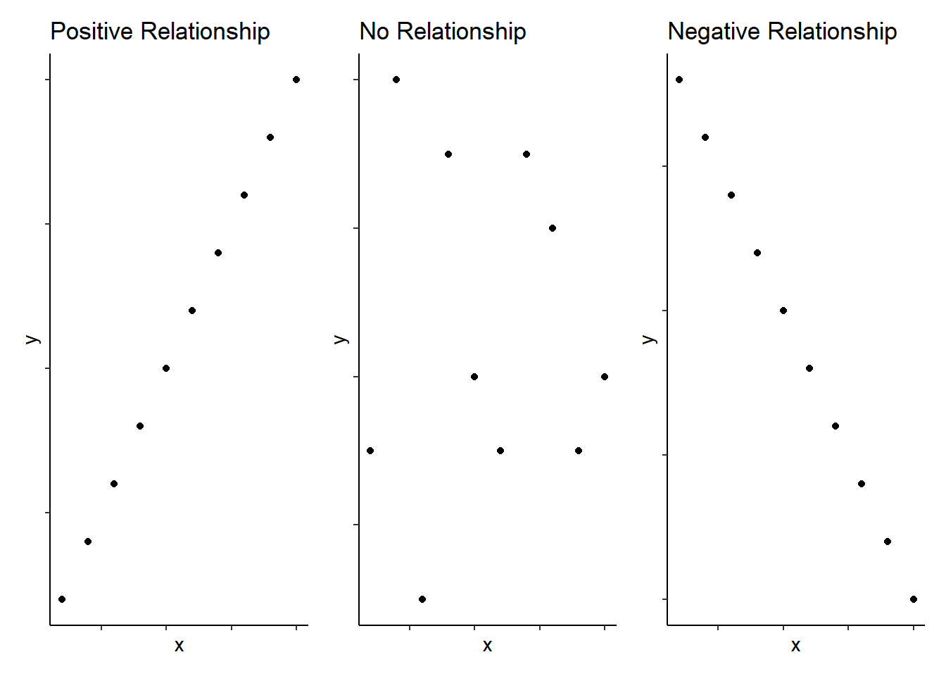
Figure 9.1: Schematic examples of extreme bivariate relationships

However, unfortunately, you may have heard people say lots of critical things about correlations:

they do not prove causality
they suffer from the bidirectional problem (A vs B is the same as B vs A)
any relationship found may be the result of an unknown third variable (e.g. murders and ice-creams)

Whilst these are true and we must be aware of them, correlations are an incredibly useful and commonly used measure in the field, so don't be put off from using them or designing a study that uses correlations. In fact, they can be used in a variety of areas. Some examples include:

looking at reading ability and IQ scores such as in Miller and Haden Chapter 11, which we will also look at today;
exploring personality traits in voices (see Phil McAleer's work on Voices);
or traits in faces (see Lisa DeBruine's work);
brain-imaging analysis looking at activation in say the amygdala in relation to emotion of faces (see Alex Todorov's work at Princeton);
social attitudes, both implicit and explicit, as Helena Paterson will discuss in her Social lectures this semester;
or a whole variety of fields where you simply measure the variables of interest.

To actually carry out a correlation is very simple and we will show you that in a little while: you can use the cor.test() function. The harder part of correlations is really wrangling the data (which you've learned to do in the first part of this book) and interpreting the data (which we will focus more on this chapter). So, we are going to run a few correlations, showing you how to do one, and asking you to perform others to give you some good practice at running and interpreting the relationships between two variables.

Note: When dealing with correlations it is better to refer to relationships and NOT predictions. In a correlation, X does not predict Y, that is really more regression which we will look at later on the book. In a correlation, what we can say is that X and Y are related in some way. Try to get the correct terminology and please feel free to pull us up if we say the wrong thing in class. It is an easy slip of the tongue to make!

In this chapter we will:

Introduce the Miller and Haden book, which we will be using throughout the rest of the book
Show you the thought process of a researcher running a correlational analysis.
Give you practice in running and writing up a correlation.

9.2 Correlations Basics

The majority of the basics activities in the first part of the chapters from now on will involve reading a chapter or two from Miller and Haden (2013) and trying out a couple of tasks. This is an excellent free textbook that we will use to introduce you to the General Linear Model, a model that underlies all the majority of analyses you have seen and will see this year - e.g., t-tests, correlations, ANOVAs (Analysis of Variance), Regression are all related and are all part of the General Linear Model (GLMs).

We will start off this chapter with some introduction to correlations.

9.2.1 Read

Chapter

Read Chapters 10 and 11 of Miller and Haden (2013).

Both chapters are really short, but give a good basis to understanding correlational analysis. Please note, in Chapter 10 you might not know some of the the terminology yet, e.g. ANOVA means Analysis of Variance and GLM means General Linear Model (Reading Chapter 1 of Miller and Haden might help). We will go into depth on these terms in the coming chapters.

9.2.2 Watch

Visualisation

Have a look at this visualisation of correlations by Kristoffer Magnusson: https://rpsychologist.com/d3/correlation/.

After having read Miller and Haden Chapter 11, use this visualisation page to visually replicate the scatterplots in Figures 11.3 and 11.4 - use a sample of 100. After that, visually replicate the scatterplots in Figure 11.5. Each time you change the correlation, pay attention to the shared variance (the overlap between the two variables) and see how this changes with the changing level of relationship between the two variables. The greater the shared variance, the stronger the relationship.
Also, try setting the correlation to r = .5 and then moving a single dot to see how one data point, a potential outlier, can change the stated correlation value between two variables

9.2.3 Play

Guess the correlation

Now that you are well versed in interpreting scatterplots (scattergrams) have a go at this online app on guessing the correlation: https://www.rossmanchance.com/applets/GuessCorrelation.html.

This is a very basic application that allows you to see how good you are at recognising different correlation strengths from the scatterplots. We would recommend you click the "Track Performance" tab so you can keep an overview of your overall bias to underestimate or overestimate a correlation.

Is this all just a bit of fun? Well, yes because stats is actually fun, and no, because it serves a purpose of helping you determine if the correlations you see in your own data are real, and to help you see if correlations in published research match with what you are being told. As you will know from the above examples one data point can lead to a misleading relationship and even what might be considered a medium to strong relationship may actually have only limited relevance in the real world. One only needs to mention Anscombe's Quartet to be reminded of the importance of visualising your data.

Anscombe (1973) showed that four sets of bivariate data (X,Y) that have the exact same means, medians, and relationships:

Table 9.1: Four bivariate datasets that have the same means, medians, standard deviations, and relationships
Group	meanX_rnd	sdX_rnd	meanY_rnd	sdY_rnd	corrs_rnd
I	9	3.317	7.501	2.032	0.816
II	9	3.317	7.501	2.032	0.816
III	9	3.317	7.500	2.030	0.816
IV	9	3.317	7.501	2.031	0.817

Can look very different when plotted:

## `geom_smooth()` using formula = 'y ~ x'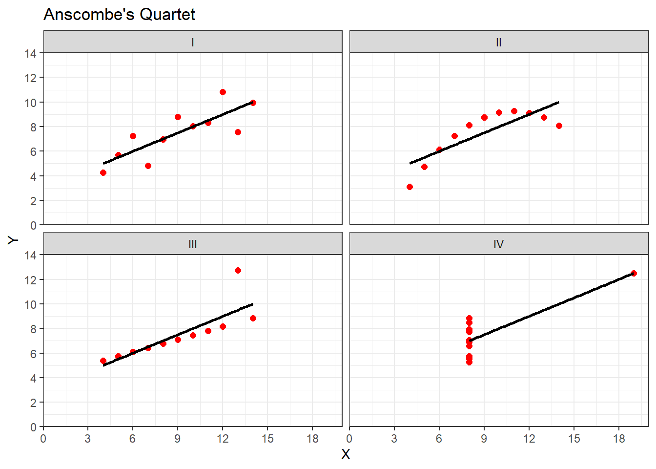

Though all datasets have a correlation of r = .82, when plotted the four datasets look very different. Grp I is a standard linear relationship where a pearson correlation would be suitable. Grp II would appear to be a non-linear relationship and a non-parametric analysis would be appropriate. Grp III again shows a linear relationship (approaching r = 1) where an outlier has lowered the correlation coefficient. Grp IV shows no relationship between the two variables (X, Y) but an oultier has inflated the correlation higher.

Figure 9.2: Though all datasets have a correlation of r = .82, when plotted the four datasets look very different. Grp I is a standard linear relationship where a pearson correlation would be suitable. Grp II would appear to be a non-linear relationship and a non-parametric analysis would be appropriate. Grp III again shows a linear relationship (approaching r = 1) where an outlier has lowered the correlation coefficient. Grp IV shows no relationship between the two variables (X, Y) but an oultier has inflated the correlation higher.

All in this is a clear example of where you should visualise your data and not to rely on just the numbers. You can read more on Anscombe's Quartet in your own time, with wikipedia (https://en.wikipedia.org/wiki/Anscombe%27s_quartet) offering a good primer and the data used for the above example.

9.3 Correlations Application

We are going to jump straight into this one! To get you used to running a correlation we will use the examples you read about in Miller and Haden (2013), Chapter 11, looking at the relationship between four variables: reading ability, intelligence, the number of minutes per week spent reading at home, and the number of minutes per week spent watching TV at home. This is again a great example of where a correlation works best because it would be unethical to manipulate these variables so measuring them as they exist in the environment is most appropriate.

Click here to download the data for today.

9.3.1 Task 1 - The Data

After downloading the data folder, unzip the folder, set your working directory appropriately, open a new R Markdown, and load in the Miller and Haden data (MillerHadenData.csv), storing it in a tibble called mh. As always, the solutions are at the end of the chapter.

Note 1: Remember that in reality you could store the data under any name you like, but to make it easier for a demonstrator to debug with you it is handy if we all use the same names.
Note 2: You will find that the instructions for tasks are sparser from now on, compared to earlier in the book. We want you to really push yourself and develop the skills you learnt previously. Don't worry though, we are always here to help, so if you get stuck, ask!
Note 3: You will see an additional data set on vaping. We will use that later on in this chapter, so you can ignore it for now.

Hint 1: We are going to need the following libraries: tidyverse, broom
Hint 2: mh <- read_csv()
Remember that, in this book, we will ALWAYS ask you to use read_csv() to load in data. Avoid using other functions such as read.csv(). Whilst these functions are similar, they are not the same.

Let's look at your data in mh - we showed you a number of ways to do this before. As in Miller and Haden, we have five columns:

Participant (Participant),
Reading Ability (Abil),
Intelligence (IQ),
Number of minutes spent reading at home per week (Home),
Number of minutes spent watching TV per week (TV).

For the exercises we will focus on the relationship between Reading Ability and IQ, but for further practice you can look at other relationships on your own.

A probable hypothesis for today could be that as Reading Ability increases so does Intelligence (but do you see the issue with causality and direction?). Or phrasing the alternative hypothesis ($H_1$) more formally, we hypothesise that the reading ability of school children, as measured through a standardized test, and intelligence, again measured through a standardized test, show a linear positive relationship. This is the hypothesis we will test today, but remember that we could always state the null hypothesis ($H_0$) that there is no relationship between reading ability and IQ.

First, however, we must check some assumptions of the correlation tests. As we have stated that we hypothesise a linear relationship, this means that we are going to be looking at the Pearson's product-moment correlation which is often just shortened to Pearson's correlation and is symbolised by the letter r.

The main assumptions we need to check for the Pearson's correlation, and which we will look at in turn, are:

Is the data interval, ratio, or ordinal?
Is there a data point for each participant on both variables?
Is the data normally distributed in both variables?
Does the relationship between variables appear linear?
Does the spread have homoscedasticity?

9.3.2 Task 2 - Interval or Ordinal

Assumption 1: Level of Measurement

Thinking Cap Point

If we are going to run a Pearson correlation then we need interval or ratio data. An alternative correlation, a non-parametric equivalent of the Pearson correlation is the Spearman correlation and it can run with ordinal, interval or ratio data. What type of data do we have?

Check your thinking: the type of data in this analysis is most probably as the data is and there is unlikely to be a true zero

are the variables continuous?
is the difference between 1 and 2 on the scale equal to the difference between 2 and 3?

9.3.3 Task 3 - Missing Data

Assumption 2: Pairs of Data

All correlations must have a data point for each participant on the two variables being correlated. This should make sense as to why - you can't correlate against an empty cell! Check that you have a data point in both columns for each participant. After that, try answering the question in Task 3. A discussion is in the solutions at the end of the chapter.

Note: You can check for missing data by visual inspection - literally using your eyes. A missing data point will show as a NA, which is short for not applicable, not available, or no answer. An alternative would be to use the is.na() function. This can be really handy when you have lots of data and visual inspection would just take too long. If for example you ran the following code:

is.na(mh)

If you look at the output from that function, each FALSE tells you that there is a data-point in that cell. That is because is.na() asks is that cell a NA; is it empty. If the cell was empty then it would come back as TRUE. As all cells have data in them, they are all showing as FALSE. If you wanted to ask the opposite question, is their data in this cell, then you would write !is.na() which is read as "is not NA". The exclamation mark ! turns the question into the opposite.

It looks like everyone has data in all the columns but let's test our skills a little whilst we are here. Answer the following questions:

How is missing data represented in a cell of a tibble?
Which code would leave you with just the participants who were missing Reading Ability data in mh:
Which code would leave you with just the participants who were not missing Reading Ability data in mh:

filter(dat, is.na(variable)) versus filter(dat, !is.na(variable))

9.3.4 Task 4 - Normality

Assumption 3: The shape of my data

The remaining assumptions are all best checked through visualisations. You could use histograms to check that the data (Abil and IQ) are both normally distributed, and you could use a scatterplot (scattergrams) of IQ as a function of Abil to check whether the relationship is linear, with homoscedasticity, and without outliers!

An alternative would be to use z-scores to check for outliers with the cut-off usually being set at around $\pm2.5SD$. You could do this using the mutate function (e.g. mutate(z = (X - mean(X))/SD(X))), but today we will just use visual checks.

Create the following figures and discuss the outputs with your group. A discussion is in the solutions at the end of the chapter.

A histogram for Ability and a histogram for IQ.
- Are they both normally distributed?
A scatterplot of IQ (IQ) as a function of Ability (Abil).
- Do you see any outliers?
- Does the relationship appear linear?
- Does the spread appear ok in terms of homoscedasticity?

ggplot(mh, aes(x = )) + geom_histogram()
ggplot(mh, aes(x = , y = )) + geom_point()
Normality: something to keep in mind is that there are only 25 participants, so how ‘normal’ do we expect relationships to be
homoscedasticity is that the spread of data points around the (imaginary) line of best fit is equal on both sides along the line; as opposed to very narrow at one point and very wide at others.
Remember these are all judgement calls!

9.3.5 Task 5 - Descriptives

Descriptives of a correlation

A key thing to keep in mind is that the scatterplot is actually the descriptive of the correlation. Meaning that in an article, or in a report, you would not only use the scatterplot to determine which type of correlation to use, but also to describe the potential relationship in regards to your hypothesis. So you would always expect to see a scatterplot in the write-up of this type of analysis

Thinking Cap Point

Looking at the scatterplot you created in Task 4, spend a couple of minutes describing the relationship between Ability and IQ in terms of your hypothesis. Remember this is a descriptive analysis at this stage, so nothing is confirmed. Does the relationship appear to be as we predicted in our hypothesis? A discussion is in the solutions at the end of the chapter.

Hint 1: We hypothesised that reading ability and intelligence were positively correlated. Is that what you see in the scatterplot?
Hint 2: Keep in mind it is subjective at this stage.
Hint 3: Remember to only talk about a relationship and not a prediction. This is correlational work, not regression.
Hint 4: Can you say something about both the strength (weak, medium, strong) and the direction (positive, negative)?

9.3.6 Task 6 - Pearson or Spearman?

The correlation

Finally we will run the correlation using the cor.test() function. Remember that for help on any function you can type ?cor.test in the console window. The cor.test() function requires:

the name of the tibble and the column name of Variable 1
the name of the tibble and the column name of Variable 2
the type of correlation you want to run: e.g. "pearson", "spearman"
the type of NHST tail you want to run: e.g. "one.sided", "two.sided"

For example, if your data is stored in dat and you are wanting a two-sided pearson correlation of the variables (columns) X and Y, then you would do:

cor.test(dat$X, dat$Y, method = "pearson", alternative = "two.sided")

where dat$X means the column X in the tibble dat. The dollar sign ($) is a way of indexing, or calling out, a specific column.

Based on your answers to Task 5, spend a couple of minutes deciding which correlation method to use (e.g., Pearson or Spearman) and the type of NHST tail to set (e.g., two.sided or one.sided). Now, run the correlation between IQ and Ability and save it in a tibble called results (hint: broom::tidy()). The solution is at the end of the chapter.

Hint 1: the data looked reasonably normal and linear so the method would be?
Hint 2: results <- cor.test(mh$Abil……, method = ….., alternative….) %>% tidy()

9.3.7 Task 7 - Interpretation

Interpreting the Correlation

You should now have a tibble called results that gives you the output of the correlation between Reading Ability and IQ for the school children measured in Miller and Haden (2013) Chapter 11. All that is left to do now is interpret the output of the correlation.

Look at results. Locate your correlation value, e.g. results %>% pull(estimate), and then answer the following questions. Again a discussion can be found at the end of the chapter.

The direction of the relationship between Ability and IQ is:
The strength of the relationship between Ability and IQ is:
Based on $\alpha = .05$ the relationship between Ability and IQ is:
Based on the output, given the hypothesis that the reading ability of school children, as measured through a standardized test, and intelligence, again through a standardized test, are positively correlated, we can say that the hypothesis:

Hint1: If Y increases as X increases then the relationship is positive. If Y increases as X decreases then the relationship is negative. If there is no change in Y as X changes then there is no relationship
Hint2: Depending on the field most correlation values greater than .5 would be strong; .3 to .5 as medium, and .1 to .3 as small.
Hint3: The field standard says less than .05 is significant.
Hint4: Hypotheses can only be supported or not supported, never proven.

9.3.8 Task 8 - The Matrix

Great, so far we have set a hypothesis for a correlation, checked the assumptions, run the correlation and interpreted it appropriately. So as you can see running the correlation is the easy bit. As in a lot of analyses it is getting your data in order, checking assumptions, and interpreting your output that is the hard part.

We have now walked you through one analysis but you can always go run more with the Miller and Haden dataset. There are six in total that could be run but watch out for Multiple Comparisons - where your False Positive Error rate (Type 1 error rate) is inflated and as such the chance of finding a significant effect is inflated by simply running numerous tests. Alternatively, we have another data set below that we want you to run a correlation on yourself but first we want to show you something that can be very handy when you want to view lots of correlations at once.

Advanced 1: Matrix of Scatterplots

Above we ran one correlation and if we wanted to do a different correlation then we would have to edit the cor.test() line and run it again. However, when you have lots of variables in a dataset, to get a quick overview of patterns, one thing you might want to do is run all the correlations at the same time or create a matrix of scatterplots at the one time. You can do this with functions from the Hmisc library - already installed in the Boyd Orr Labs. We will use the Miller and Haden data here again which you should still have in a tibble called mh.

First, we need to get rid of the Participant column as we don't want to correlate that with anything. It won't tell us anything. Copy and run the below line of code

library("Hmisc")
library("tidyverse")
mh <- read_csv("MillerHadenData.csv") %>% select(-Participant)

Now run the following line. The pairs() function from the Hmisc library creates a matrix of scatterplots which you can then use to view all the relationships at the one time.

pairs(mh)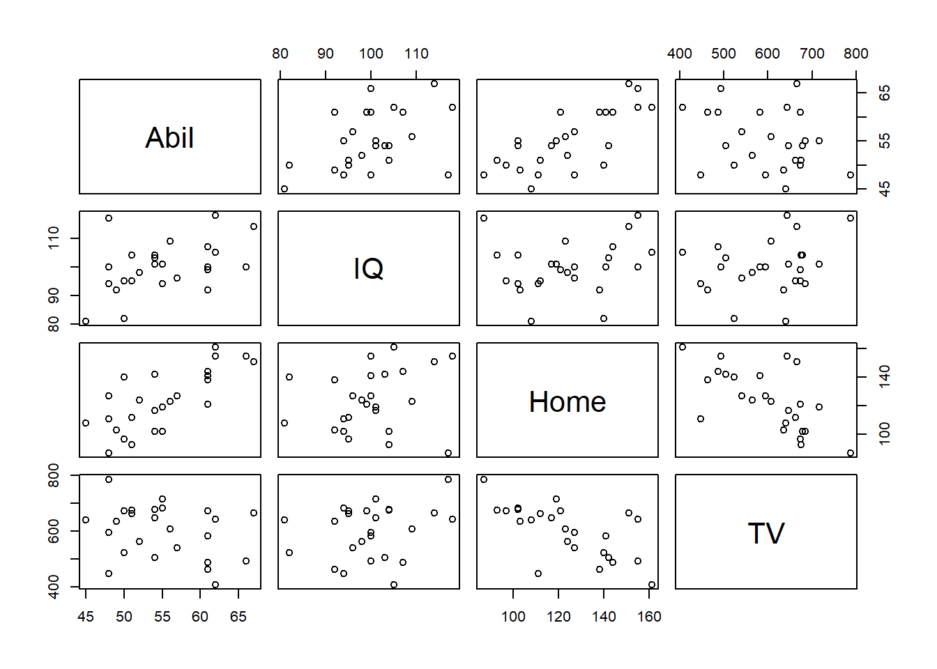

Figure 9.3: Matrix of Correlation plots of Miller and Haden (2013) data

And the rcorr() function creates a matrix of correlations and p-values. But watch out, it only accepts the data in matrix format. Run the following two lines of code.

mh_mx <- as.matrix(mh)
rcorr(mh_mx, type = "pearson")

##       Abil   IQ  Home    TV
## Abil  1.00 0.45  0.74 -0.29
## IQ    0.45 1.00  0.20  0.25
## Home  0.74 0.20  1.00 -0.65
## TV   -0.29 0.25 -0.65  1.00
## 
## n= 25 
## 
## 
## P
##      Abil   IQ     Home   TV    
## Abil        0.0236 0.0000 0.1624
## IQ   0.0236        0.3337 0.2368
## Home 0.0000 0.3337        0.0005
## TV   0.1624 0.2368 0.0005

After running the above lines, spend a few minutes answering the following questions. The first table outputted is the correlation values and the second table is the p-values.

Why do the tables look symmetrical around a blank diagonal?
What is the strongest positive correlation?
What is the strongest negative correlation?

Hint1: There is no hint, this is just a cheeky test to make sure you have read the correlation chapter in Miller and Haden, like we asked you to! :-) If you are unsure of these answers, the solutions are at the end of the chapter.

9.3.9 Task 9 - Power Calculations

In the previous chapter (Chapter 8), we looked at power calculations in relation to t-tests. Now, let’s look at power calculations in the context of correlations.

For correlations, we are going to take a similar approach. However, instead of using the pwr.t.test() function, we will use the pwr.r.test() function. The structure of this function is very similar to pwr.t.test() and works on the same leave-one-out principle:

n - Number of observations/participants
r - Correlation coefficient (the effect size of interest)
sig.level or $\alpha$
power or $1-\beta$
alternative - a character string specifying the alternative hypothesis, must be one of two.sided (default), greater (a positive correlation) or less (a negative correlation).

1. Sample size for a correlation

Before running the next line of code, use the library() function to load the pwr package.

Assuming you are interested in detecting a minimum correlation of r = .4 (in either direction), what would be the minimum number of participants you would need for a correlation analysis, assuming power = .8, $\alpha$ = .05?

Using a pipeline, store the answer as a single, rounded value called sample_size_r (i.e. use pluck() %>% ceiling()).

Enter the minimum number of participants you would need in this correlation:

2. Effect size for a correlation analysis

You run a correlation analysis with 50 participants and the standard power and alpha levels and you have hypothesised a positive correlation. What would be the minimum effect size you can reliably detect? Answer the following questions to check your answers. The solutions are at the bottom if you need them:
Based on the information given, what will you set alternative as in the function?
Based on the output, enter the minimum effect size you can reliably detect in this test, rounded to two decimal places:
According to Cohen (1988), the effect size for this correlation is
Say you run the study and find that the effect size determined is r = .24. Given what you know about power, select the statement that is true:

the study is sufficiently powered as the analysis indicates you can only detect effect sizes smaller than r = .24the study is underpowered as the analysis indicates you can only detect effect sizes larger than r = .34

9.3.10 Task 10 - Attitudes to Vaping

Advanced 2: Attitudes towards Vaping

Great work so far! Now we really want to see what you can do yourself. As we mentioned earlier, in the data folder there is another file called VapingData.csv. This data comes from a data set looking at implicit and explicit attitudes towards vaping.

Explicit attitudes were measured via a questionnaire where higher scores indicated a positive attitude towards vaping.
Implicit attitudes were measured through an Implicit Association Test (IAT) using images of Vaping and Kitchen utensils and associating them with positive and negative words.

The IAT works on the principle that associations that go together (that are congruent, e.g. warm and sun) should be quicker to respond to than associations that do not go together (that are incongruent, e.g. warm and ice). You can read up more on the procedure at a later date on the Noba Project https://nobaproject.com/modules/research-methods-in-social-psychology which has a good description of the procedure under the section "Subtle/Nonsconscious Research Methods".

For this exercise, you need to know that "Block 3" in the experiment tested reaction times and accuracy towards congruent associations, pairing positive words with Kitchen utensils and negative words with Vaping. "Block 5" in the experiment tested reaction times and accuracy towards incongruent associations, pairing positive words with Vaping and negative words with Kitchen Utensils. As such, if reaction times were longer in "Block 5" than in "Block 3" then people are considered to hold the view that Vaping is negative (i.e., congruent associations are quicker than incongruent associations). However, if reaction times were quicker in "Block 5" than in "Block 3" then people are considered to hold the view that Vaping is positive (i.e., incongruent associations were quicker than congruent associations). The difference between reaction times in "Block 5" and "Block 3" is called the participants IAT score.

Load in the data in VapingData.csv and analyse it to test the hypothesis that Implicit and Explicit attitudes towards Vaping are positively related. Here are some pointers, hints and tips. Again, the solutions walk you through each step, but it will help you to try the steps yourself first. Think through each step. Sometimes you will need to think backwards, what do I want my tibble to look like. You can do all of these steps. This is nothing new.

After loading in the data, start by looking at the data. You have 8 columns. Reaction times and Accuracy scores for Blocks 3 and 5 as well as the Explicit Vaping Questionnaire scores, Gender and Age, for each participant.
Accuracy was calculated as proportion and as such can't go above 1. Participants entered their own data so some might have made a mistake. Remove participants who had an accuracy greater than 1 in either Block 3 or Block 5 as we are unclear on the accuracy of these values.
We also only want participants that were paying attention so best remove anybody whose average accuracy score across Blocks 3 and 5 was less than 80%. Note - this value is arbitrary and if you wanted, in your own experiment, you could use a more relaxed or strict cut-off based on other studies or guidance. Note that these decisions should be set out at the start of your research as part of your pre-registration or as part of your Registered Report. Finally, in this instance, remember, the values are in proportions not percentages (so 80% will be .8).
Now create an IAT score for participants by subtracting Block 3 reaction times (RT) away from Block 5 reaction times e.g $Block5 - Block3$. Use the information above to understand how the scores relate to attitudes.
Create a descriptives summary of the number of people, the mean RT and Vaping Questionnaire Score. Why might these averages be useful? Why are averages not always useful in correlations?
Check your assumptions of correlations as we did above and descriptives, thinking about how it compares to the hypothesis.
Run the appropriate correlation based on your assumptions and interpret the output.

libraries might include tidyverse and broom
Hint Step 1: read_csv()
Hint Step 2: filter(Accuracy < 1 OR Accuracy <= 1 OR Accuracy > 1 OR Accuracy >= 1)
Hint Step 3: average accuracy: mutate(data, name = (1 + 2)/2) %>% filter(name > …)
Hint Step 4: RT: mutate(data, nom = 1 - 2)
Hint Step 5: descriptives <- summarise()
Hint Step 6: assumptions would be type of data, normality, linear relationship, homoscedasicity, data points for everyone!
Hint Step 7: results <- cor.test(method = “pearson”)?

Excellent work, who would have thought that about Explicit and Implicit attitudes towards Vaping?

9.4 Practice Your Skills

The purpose of this exercise is to test your ability to run and interpret a correlation for yourself, as shown in this chapter, but at the same time get you to think about all the skills you learnt previously. Most of the hard work is in the data wrangling; running the actual analysis, much like with t-tests, is very straightforward. Remember to refer back to previous chapters when stuck.

In order to complete these tasks you will need to download the data .csv file and the .Rmd file, which you need to edit, titled GUID_L2_Ch9_PracticeSkills.Rmd. These can be downloaded within a zip file from the below link. Download the Exercises .zip file from here.

In that zip file, you will also find the activity html file where you can check the table and figure to be reproduced for tasks 8 and 9.

Once downloaded and unzipped you should create a new folder that you will use as your working directory; put the data file and the .Rmd file in that folder and set your working directory to that folder through the drop-down menus at the top. The .Rmd file itself will currently knit as there are no errors in the code and this is a good test that you can perform from time to time to make sure that there are still no errors in your code. Obviously this doesn't mean that all your answers are correct; it just means that the code is error free.

As in the previous exercises there are a number of code chunks already set up. The code chunks will require entering a number or entering and adjusting code that you have practiced in the chapters. Follow the instructions on what to edit in each code chunk. This will often be entering code based on what we have covered up until this point.

Background The backdrop for the exercise is the following study:

Dawtry, R. J., Sutton, R. M., & Sibley, C. G. (2015). Why wealthier people think people are wealthier, and why it matters: From social sampling to attitudes to redistribution. Psychological Science, 26, 1389-1400. Available on through this link with your VPN switched on

The abstract of Dawtry, Sutton and Sibley (2015) reads:

The present studies provide evidence that social-sampling processes lead wealthier people to oppose redistribution policies. In samples of American Internet users, wealthier participants reported higher levels of wealth in their social circles (Studies 1a and 1b). This was associated, in turn, with estimates of higher mean wealth in the wider U.S. population, greater perceived fairness of the economic status quo, and opposition to redistribution policies. Furthermore, mods from a large-scale, nationally representative New Zealand survey revealed that low levels of neighborhood-level socioeconomic deprivation - an objective index of wealth within participants' social circles - mediated the relation between income and satisfaction with the economic status quo (Study 2). These findings held controlling for relevant variables, including political orientation and perceived self-interest. Social-structural inequalities appear to combine with social-sampling processes to shape the different political attitudes of wealthier and poorer people.

And is summarised by the Open Stats Lab as

In this research, Dawtry, Sutton, and Sibley (2015) wanted to examine why people differ in their assessments of the increasing wealth inequality within developed nations. Previous research reveals that most people desire a society in which the overall level of wealth is high and that wealth is spread somewhat equally across society. However, support for this approach to income distribution changes across the social strata. In particular, wealthy people tend to view society as already wealthy and thus are satisfied with the status quo, and less likely to support redistribution. In their paper Dawtry et al., (2015) sought to examine why this is the case. The authors propose that one reason wealthy people tend to view the current system is fair is because their social-circle is comprised of other wealthy people, which biases their perceptions of wealth, which leads them to overestimate the mean level of wealth across society.

To test this hypothesis, the authors conducted a study with 305 participants, recruited from an online participant pool. Participants reported their own annual household income, the income level of those within their own social circle, and the income for the entire population. Participants also rated their perception of the level of equality/inequality across their social circle and across society, their level of satisfaction with and perceived fairness of the current system (measured using two scales), their attitudes toward redistribution of wealth (measured using a four-item scale), and their political preference.

The Open Stats Lab has an activity for this paper already set up that you can work through later for your own skills development. Here we will use an amended version so pay close attention to the instructions in this assignment and do specifically as each task asks. Today we will be running a correlation between a measure of Fairness and Satisfaction versus a measure of Support for Redistribution.

9.5 Solutions to Questions

Below you will find the solutions to the questions for the activities for this chapter. Only look at them after giving the questions a good try and speaking to the tutor about any issues.

9.5.1 Correlations Application

9.5.1.1 Task 1

Loading in the data and the two libraries needed
Good point to remind you that:
- we use read_csv() to load in data
- the order that libraries are read in is important. If there are any conflicts in terms of libraries then the last library that is loaded will be the functions you are using.

library("broom")
library("tidyverse")
mh <- read_csv("MillerHadenData.csv")

Return to Task

9.5.1.2 Task 2

Actually the information within the textbook is unclear as to whether the data is interval or ordinal so we have accepted both as you could make a case for both arguments. A quick Google search will show just as many people who think that IQ is interval as think it is ordinal. In terms of Reading Ability, again we probably don't know enough information about this scale to make a clear judgement but it is at least ordinal and could well be interval.

Return to Task

9.5.1.3 Task 3

Missing data is represented by NA. It stands for Not Available but is a very good way of improving your Scottish accent. For example, "is that a number" can be replied with "NA!".
If you want to keep everybody from the whole dataset that has a score for Ability you would use:

filter(mh, !is.na(Abil))

Participant	Abil	IQ	Home	TV
1	61	107	144	487
2	56	109	123	608
3	45	81	108	640
4	66	100	155	493
5	49	92	103	636
6	62	105	161	407
7	61	92	138	463
8	55	101	119	717
9	62	118	155	643
10	61	99	121	674
11	51	104	93	675
12	48	100	127	595
13	50	95	97	673
14	50	82	140	523
15	67	114	151	665
16	51	95	112	663
17	55	94	102	684
18	54	103	142	505
19	57	96	127	541
20	54	104	102	678
21	52	98	124	564
22	48	117	87	787
23	61	100	141	582
24	54	101	117	647
25	48	94	111	448

Alternatively, if you want to keep everybody from the whole dataset that does not have a score for Ability you would use:

filter(mh, is.na(Abil))

Participant	Abil	IQ	Home	TV

Remember that you would need to store the output of this step, so really it would be something like mh <- filter(mh, !is.na(Abil))

Return to Task

9.5.1.4 Task 4

Reading ability data appears as normal as expected for 25 participants. Hard to say how close to normality something should look when there are so few participants.

ggplot(mh, aes(x = Abil)) + 
  geom_histogram(binwidth = 5) +
  theme_bw()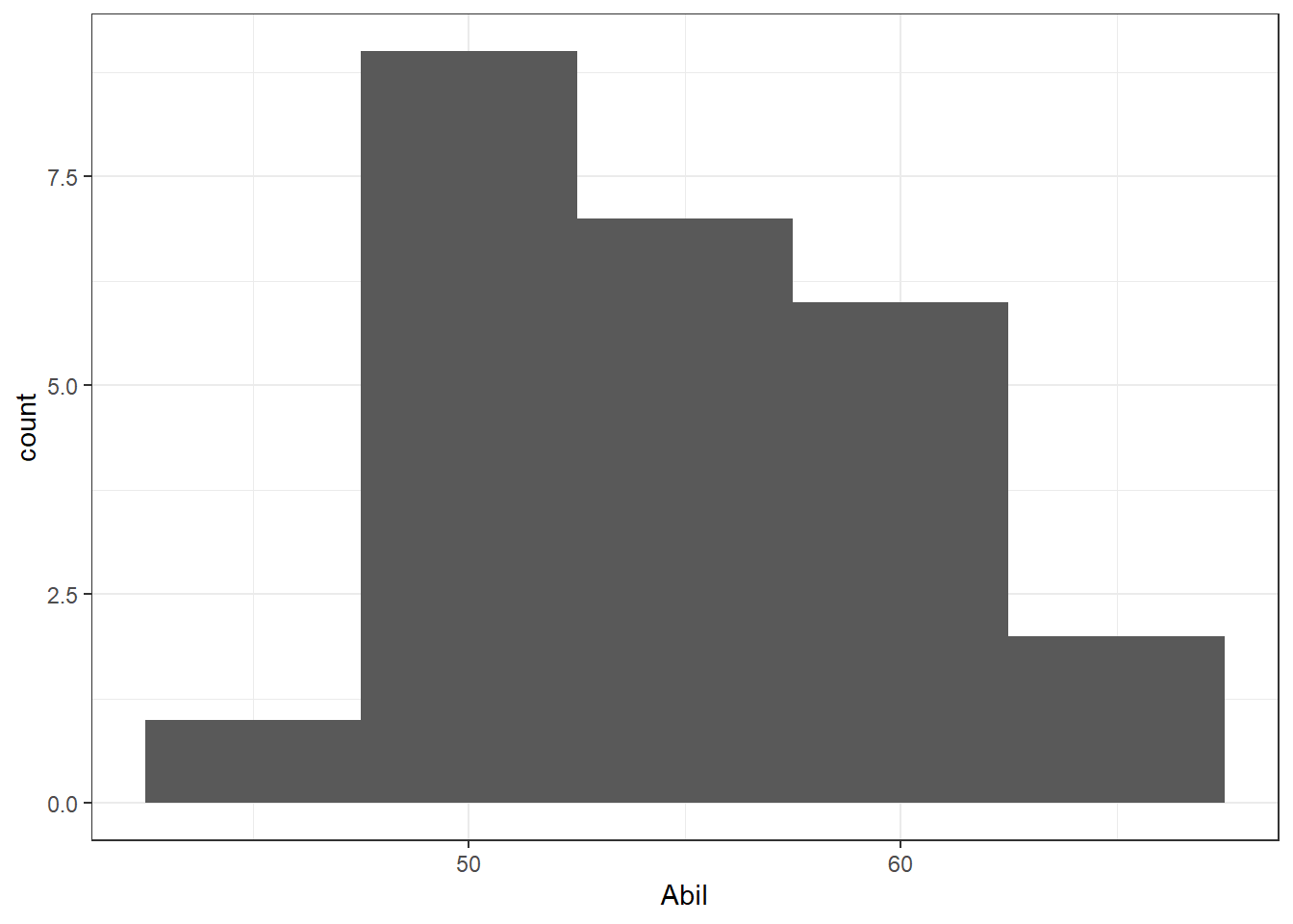

Figure 9.4: Histogram showing the distribution of Reading Ability Scores from Miller and Haden (2013)

IQ data appears as normal as expected for 25 participants

ggplot(mh, aes(x = IQ)) + 
  geom_histogram(binwidth = 5) +
  theme_bw()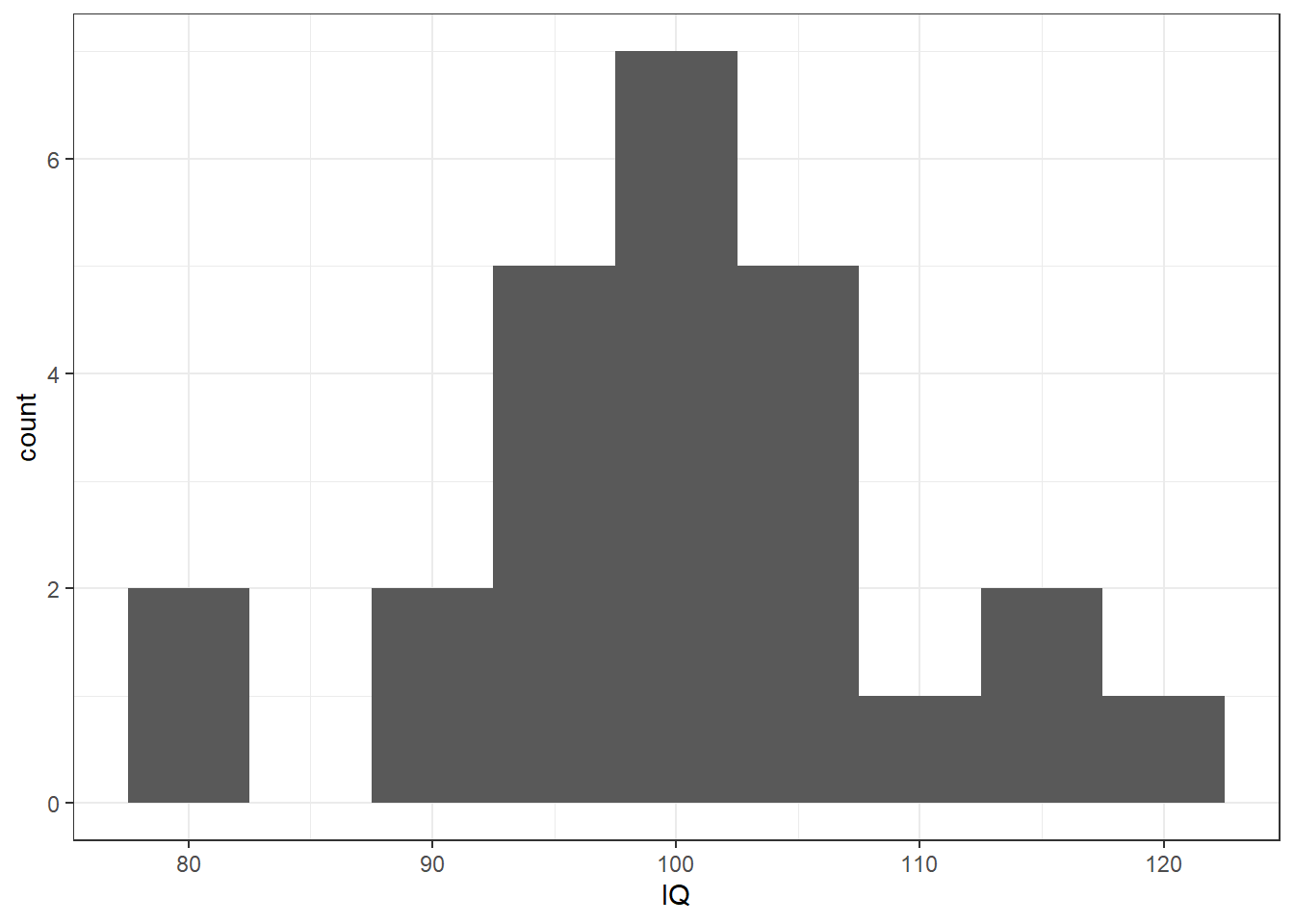

Figure 9.5: Histogram showing the distribution of IQ Scores from Miller and Haden (2013)

The relationship between reading ability and IQ scores appears appears linear and with no clear outliers. Data also appears homeoscedastic.
We have added the geom_smooth() function to help clarify the line of best fit (also know as the regression line or the slope).

ggplot(mh, aes(x = Abil, y = IQ)) + 
  geom_point() +
  geom_smooth(method = "lm", se = FALSE) +
  theme_bw()

## `geom_smooth()` using formula = 'y ~ x'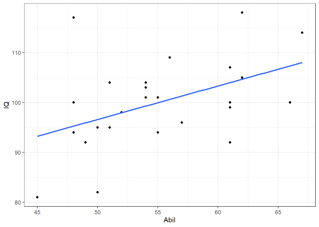

Figure 9.6: Scatterplot of IQ scores as a function of Reading Ability from Miller and Haden (2013) data

Return to Task

9.5.1.5 Task 5

Based on the scatterplot we might suggest that as reading ability scores increase, IQ scores also increase and as such it would appear that our data is inline with our hypothesis that the two variables are positively correlated. This appears to be a medium strength relationship.

Return to Task

9.5.1.6 Task 6

We are going to run a pearson correlation as we would argue the data is interval and the relationship is linear.
The correlation would be run as follows - tidying it into a nice and usable table.

results <- cor.test(mh$Abil, 
                    mh$IQ, 
                    method = "pearson", 
                    alternative = "two.sided") %>% 
  broom::tidy()

The output of the table would look as follows:

Table 9.2: Table 9.3: The correlation output of the Reading Ability and IQ relationship.
estimate	statistic	p.value	parameter	conf.low	conf.high	method	alternative
0.451	2.425	0.024	23	0.068	0.718	Pearson's product-moment correlation	two.sided

Return to Task

9.5.1.7 Task 7

In the Task 6 output:

The correlation value (r) is stored in estimate
The degrees of freedom (N-2) is stored in parameter
The p-value is stored in p.value
And statistic is the t-value associated with this analysis as correlations use the t-distribution (same as in Chapters 6, 7 and 8) to determine probability of an outcome.
Remember that we can use the pull() function to get individual values as shown here.

pvalue <- results %>% 
  pull(p.value) %>% 
  round(3)

df <- results %>% 
  pull(parameter)

correlation <- results %>% 
  pull(estimate) %>% 
  round(2)

And we can use that information to write-up the following using inline coding for accuracy:

A pearson correlation found reading ability and intelligence to be positively correlated with a medium to strong relationship, (r(`r df`) = `r correlation`, p = `r pvalue`). As such we can say that our hypothesis is supported and that there appears to be a relationship between reading ability and IQ in that as reading ability increases so does intelligence.

Which when knitted would read as:

A pearson correlation found reading ability and intelligence to be positively correlated with a medium to strong relationship, (r(23) = 0.45, p = 0.024). As such we can say that our hypothesis is supported and that there appears to be a relationship between reading ability and IQ in that as reading ability increases so does intelligence.

Return to Task

9.5.1.8 Task 8

The table looks the same across the diagonal because the correlation of e.g. Abil vs Abil is not shown, and the correlation of Abil vs Home is the same as the correlation of Home vs Abil.
The strongest positive correlation is between the number of minutes spend reading at home (Home) and Reading Ability (abil), r(23) = .74, p < .001.
The strongest negative correlation is between the number of minutes spend reading at home (Home) and minutes spent watching TV per week (TV), r(23) = -.65, p < .001.

Return to Task

9.5.1.9 Task 9

1. Sample size for a correlation

library(pwr)

sample_size_r <- pwr.r.test(r = .4, 
                            sig.level = .05, 
                            power = .8, 
                            alternative = "two.sided") %>%
  pluck("n") %>% 
  ceiling()

2. Effect size for a correlation analysis

pwr.r.test(n = 50,
           sig.level = .05, 
           power = .8, 
           alternative = "greater") %>%
  pluck("r") %>%
  round(2)

## [1] 0.34

Return to Task

9.5.1.10 Task 10

Step 1

Reading in the Vaping Data using read_csv()

dat <- read_csv("VapingData.csv")

Steps 2 to 4

The main wrangle of parts 2 to 4

dat <- dat %>% 
  filter(IAT_BLOCK3_Acc <= 1) %>%
  filter(IAT_BLOCK5_Acc <= 1) %>%
  mutate(IAT_ACC = (IAT_BLOCK3_Acc + IAT_BLOCK5_Acc)/2) %>%
  filter(IAT_ACC > .8) %>%
  mutate(IAT_RT = IAT_BLOCK5_RT - IAT_BLOCK3_RT)

Step 5

It is always worth thinking about which averages are informative and which are not.
- Knowing the average explicit attitude towards vaping could well be informative.
- In contrast, if you are using an ordinal scale and people use the whole of the scale then the average may just tell you the middle of the scale you are using - which you already know and really isn't that informative. So it is always worth thinking about what your descriptives are calculating.

descriptives <- dat %>% summarise(n = n(),
                          mean_IAT_ACC = mean(IAT_ACC),
                          mean_IAT_RT = mean(IAT_RT),
                          mean_VPQ = mean(VapingQuestionnaireScore, 
                                          na.rm = TRUE))

Step 6

A couple of visual checks of normality through histograms

ggplot(dat, aes(x = VapingQuestionnaireScore)) + 
  geom_histogram(binwidth = 10) +
  theme_bw()

## Warning: Removed 11 rows containing non-finite outside the scale range
## (`stat_bin()`).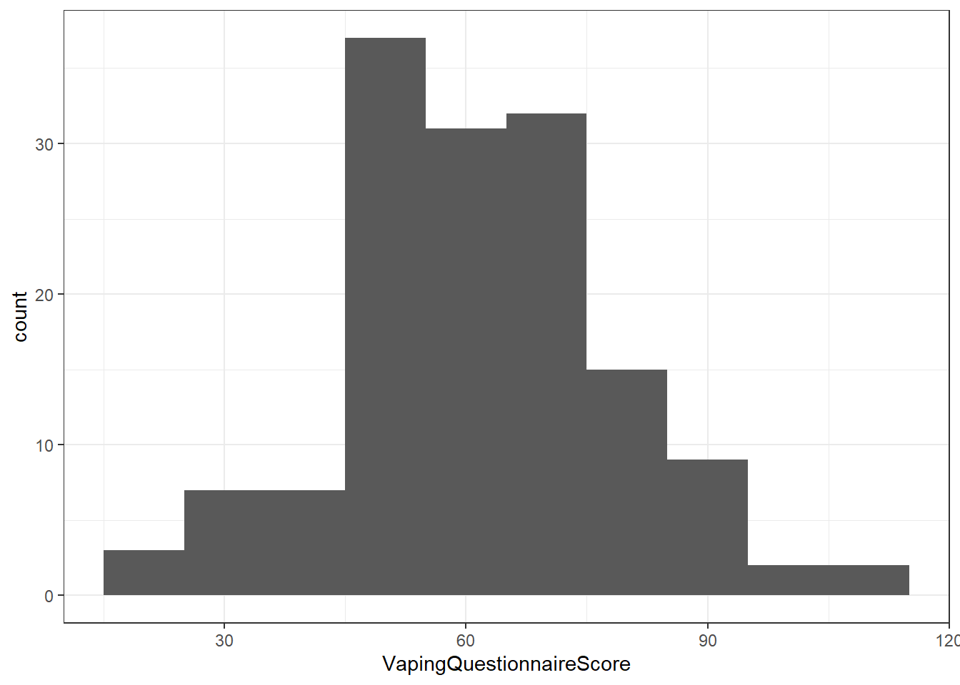

Figure 9.7: Histogram showing the distribution of Scores on the Vaping Questionnaire (Explicit)

ggplot(dat, aes(x = IAT_RT)) + 
  geom_histogram(binwidth = 10) +
  theme_bw()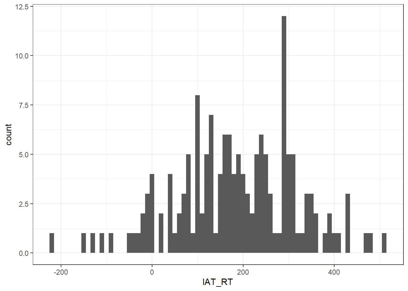

Figure 9.8: Histogram showing the distribution of IAT Reaction Times (Implicit)

A check of the relationship between reaction times on the IAT and scores on the Vaping Questionnaire.
Remember that, often, the scatterplot is considered the descriptive of the correlation, hence why you see them including in journal articles to support the stated relationship.
The scatterplot can be used to make descriptive claims about the direction of the relationship, the strength of the relationship, whether it is linear or not, and to check for outliers and homeoscedasticity.

ggplot(dat, aes(x = IAT_RT, y = VapingQuestionnaireScore)) + 
  geom_point() + 
  theme_bw()

## Warning: Removed 11 rows containing missing values or values outside the scale range
## (`geom_point()`).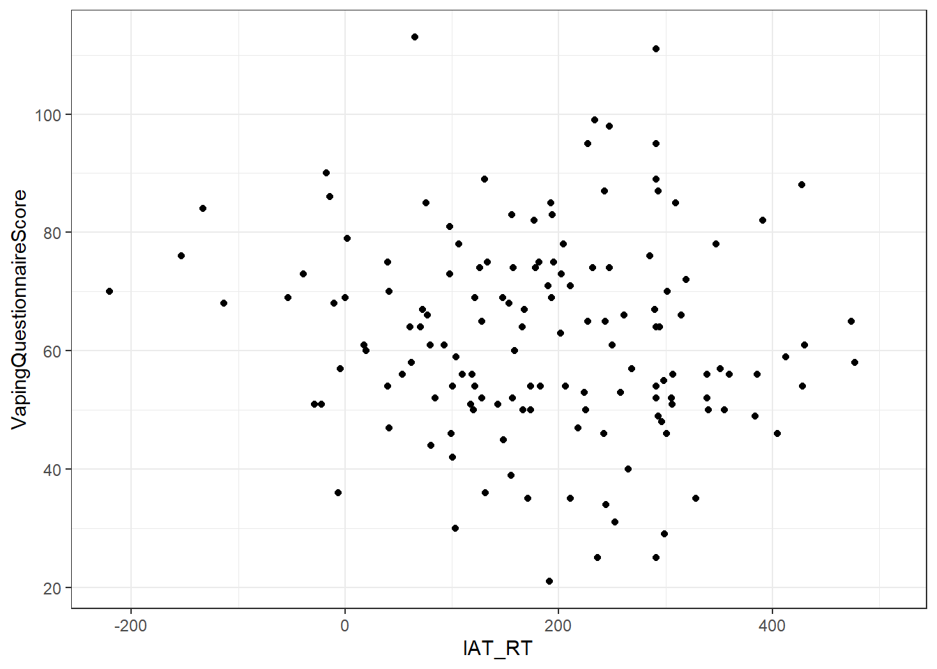

Figure 9.9: A scatterplot showing the relationship between implicit IAT reaction times (x) and explicit Vaping Questionnaire Scores (y)

A quick look at the data reveals some people do not have a Vaping Questionnaire score and some don't have an IAT score. The correlation only works when people have a score on both factors so we remove all those that only have a score on one of the factors.

dat <- dat %>% 
  filter(!is.na(VapingQuestionnaireScore)) %>% 
  filter(!is.na(IAT_RT))

Step 7

The analysis:

results <- cor.test(dat$VapingQuestionnaireScore, 
                    dat$IAT_RT, 
                    method = "pearson") %>% 
  broom::tidy()

And extracting the values:

correlation <- results %>% 
  pull(estimate)

df <- results %>% 
  pull(parameter)

pvalue <- results %>% 
  pull(p.value)

With inline coding:

Testing the hypothesis that there would be a relationship beween implicit and explicit attitudes towards vaping, a pearson correlation found no significant relationship between IAT reaction times (implicit attitude) and answers on a Vaping Questionnaire (explicit attitude), r(`r df`) = `r correlation`, p = `r pvalue`. Overall this suggests that there is no direct relationship between implicit and explicit attitudes when relating to Vaping and as such our hypothesis was not supported; we cannot reject the null hypothesis.

and appears as when knitted:

Testing the hypothesis that there would be a relationship beween implicit and explicit attitudes towards vaping, a pearson correlation found no significant relationship between IAT reaction times (implicit attitude) and answers on a Vaping Questionnaire (explicit attitude), r(143) = -0.1043797, p = 0.2115059. Overall this suggests that there is no direct relationship between implicit and explicit attitudes when relating to Vaping and as such our hypothesis was not supported; we cannot reject the null hypothesis.

Remember though that r-values and p-values are often rounded to three decimal places, so a more appropriate write up would be:

Testing the hypothesis that there would be a relationship beween implicit and explicit attitudes towards vaping, a pearson correlation found no significant relationship between IAT reaction times (implicit attitude) and answers on a Vaping Questionnaire (explicit attitude), r(143) = -.104, p = .212. Overall this suggests that there is no direct relationship between implicit and explicit attitudes when relating to Vaping and as such our hypothesis was not supported; we cannot reject the null hypothesis.

9.5.2 Practice Your Skills

Check your work against the solution to the tasks here: Chapter 9 Practice Your Skills Solution.

Return to Task

9.6 Additional Material

Below is some additional material that might help you understand correlations a bit more and some additional ideas.

Checking for outliers with z-scores

We briefly mentioned in the above activities that you could use z-scores to check for outliers, instead of visual inspection. We have covered this in lectures and it works for any interval or ratio dataset, and not just ones for correlations, but we will demonstrate it here using the IQ data from Miller and Haden. First, lets get just the IQ data.

mh_IQ <- mh %>% 
  select(IQ)

A z-score is just a standardised value based on the mean ($\mu$) and standard deviation (SD or $\sigma$, proonounced "sigma") of the sample it comes from. The formula for a z-score is:

\[z = \frac{x - \mu}{\sigma}\]

Using z-scores is away of effectively converting your data onto the Normal Distribution. As such, because of known cut-offs from the Normal Distribution (e.g., 68% of data between $\pm1SD$, etc - See Chapter 4), we can use that information to determine a value as an outlier. To do it, you convert all the data within your variable into their respective z-score and if any of the values fall above or below your cut-off then they are considered an outlier.

mh_IQ_z <- mh_IQ %>%
  mutate(z_scores = (IQ - mean(IQ))/sd(IQ))

Which will give us the following data (showing only the first 6 rows):

Table 9.4: Raw IQ data and z-scored IQ data from Miller and Haden
IQ	z_scores
107	0.7695895
109	0.9907359
81	-2.1053138
100	-0.0044229
92	-0.8890086
105	0.5484431
92	-0.8890086

And if you run through the data you will see a whole range of z-scores ranging from -2.1053138 to 1.9858948. During the class we said that we would use a cut-off of $\pm2.5SD$ and you can see from the range of the IQ z-scores that there is no value above that, so we have no outliers. Which you could confirm with the following code:

mh_IQ_z %>% filter(abs(z_scores) > 2.5) %>% count() %>% pull(n)

Which if you run that code, you can see we have 0 outliers. This also demonstrates however why you must stipulate your cut-offs in advance - otherwise you might fall foul of adjusting your data to fit your own predictions and hiding your decision making in the numerous researcher degrees of freedom that exist. For example, say you run the above analysis and see no outliers but don't find the result you want/expect/believe should be there. A questionable research practice would be now to start adjusting your z-score cut-off to different values to see what difference that makes. For instance, had we said the cut-off was more stringent at $\pm2SD$ we would have found 1 outlier.

So the two take-aways from this are:

How to spot outliers using z-scores.
You must set your exclusion criteria in advance of running your analysis.

A different approach to making a correlation table

In the above activities, Task 8, we looked at making a table of correlation functions. It was a bit messy and there is actually an alternative approach that we can use, with some useful additional functions. This makes use of the corrr package which you may need to install onto your laptop if you want to follow along.

Here is the code below that you can try out and explore yourself. The main functions are correlate(), shave(), and fashion():

correlate() runs the correlations and can be changed between pearson, spearman, etc. The quiet argument just removes some information reminders that we dont really need. Switch it to FALSE to see what happens. A nice aspect of this function is that the default is to only use complete rows but you can alter that.
shave() can be used to convert one set of correlation values that are showing the same test to NAs. For example, the bottom half of the table just reflects the top half of the table so we can convert one half. The default is to convert the upper half of the table.
fashion() can be used to tidy up the table in terms of removing NAs, leading zeros, and for setting the number of decimal places.

The code would look like this:

library(corrr)

mh <- read_csv("MillerHadenData.csv")

mh %>% 
  select(-Participant) %>%
  correlate(method = "pearson", quiet = TRUE) %>%
  shave() %>%
  fashion(decimals = 3, leading_zeros = FALSE)

Which if you then look at the ouput you get this nice clean correlation matrix table shown below.

term	Abil	IQ	Home
Abil
IQ	.451
Home	.744	.202
TV	-.288	.246	-.648

So that is a bit of a nicer approach than the one shown in Task 8, and gives you more control over the output of your correlation matrix table. However, the downside of this approach, and the reason we didn't use it above is because this approach does not show you the p-values that easily. In fact, it doesn't show you them at all and you need to do a bit more work. You can read more about using the corrr package in this webpage by the author of the package: https://drsimonj.svbtle.com/exploring-correlations-in-r-with-corrr

Comparing Correlations

One step that is often overlooked when working with correlations and a data set with numerous variables, is to compare whether the correlations are significantly different from each other. For example, say you are looking at whether there is a relationship between height and attractiveness in males and in females. You run the two correlations and find one is a stronger relationship than the other. Many would try to conclude that that means there is a significantly stronger relationship in one gender than the other. However that has not been tested. It can be tested though. We will quickly show you how, but this paper will also help the discussion: Diedenhofen and Musch (2015) cocor: A Comprehensive Solution for the Statistical Comparison of Correlations. PLOS ONE 10(6): e0131499. https://journals.plos.org/plosone/article?id=10.1371/journal.pone.0121945

As always we need the libraries first. You will need to install the cocor package on to your laptop.

library(cocor)
library(tidyverse)

Now we are going to walk through three different examples just to show you how it would work in different experimental designs. You will need to match the values in the code with the values in the text to make full sense of these examples. We will use examples from work on faces, voices and personality traits that you will encounter later in this book.

Comparing correlation of between-subjects designs (i.e., independent-samples)

Given the scenario of males voice pitch and height (r(28) = .89) and female voice pitch and height (r(28) = .75) can you say that the difference between these correlations is significant?

As these correlations come from two different groups - male voices and female voices - we used the cocor.indep.groups() function.

Note: As the df of both groups is 28, this means that the N is 30 of both groups (based on N = df-2)

compare1 <- cocor.indep.groups(r1.jk = .89, 
                               r2.hm = .75, 
                               n1 = 30, 
                               n2 = 30)

Gives the output of:

## 
##   Results of a comparison of two correlations based on independent groups
## 
## Comparison between r1.jk = 0.89 and r2.hm = 0.75
## Difference: r1.jk - r2.hm = 0.14
## Group sizes: n1 = 30, n2 = 30
## Null hypothesis: r1.jk is equal to r2.hm
## Alternative hypothesis: r1.jk is not equal to r2.hm (two-sided)
## Alpha: 0.05
## 
## fisher1925: Fisher's z (1925)
##   z = 1.6496, p-value = 0.0990
##   Null hypothesis retained
## 
## zou2007: Zou's (2007) confidence interval
##   95% confidence interval for r1.jk - r2.hm: -0.0260 0.3633
##   Null hypothesis retained (Interval includes 0)

You actually get two test outputs with this function: Fisher's Z and Zou's Confidence Interval. The one most commonly used is Fisher's Z so we will look at that one. As the p-value of the comparison between the two correlations, p = .1, is greater than p = .05, then this tells us that we have cannot reject the null hypothesis that there is no significant difference between these two correlations and they are of similar magnitude - i.e. the correlation is similar in both groups.

You would report this outcome along the lines of, "despite the correlation between male voice pitch and height was found to be stronger than the same relationship in female voices, Fisher's Z suggested that this was not a significant difference (Z = 1.65, p = .1)"

Within-Subjects (i.e., dependent samples) with common variable

What about the scenario where you have 30 participants rating faces on the scales of trust, warmth and likability, and we want to know if the relationship between trust and warmth (r = .89) is significantly different than the relationship between trust and likability (r = .8).

As this data comes from the same participants, and there is crossover/overlap in traits - i.e. one trait appears in both correlations of interest - then we will use the cocor.dep.groups.overlap(). To do this comparison we also need to know the relationship between the remaining correlation of warmth and likability (r = .91).

Note: The order of input of correlations matters. See ?cocor.dep.groups.overlap() for help.

compare2 <- cocor.dep.groups.overlap(r.jk = .89, 
                                     r.jh = .8, 
                                     r.kh = .91, 
                                     n = 30)

Gives the output of:

## 
##   Results of a comparison of two overlapping correlations based on dependent groups
## 
## Comparison between r.jk = 0.89 and r.jh = 0.8
## Difference: r.jk - r.jh = 0.09
## Related correlation: r.kh = 0.91
## Group size: n = 30
## Null hypothesis: r.jk is equal to r.jh
## Alternative hypothesis: r.jk is not equal to r.jh (two-sided)
## Alpha: 0.05
## 
## pearson1898: Pearson and Filon's z (1898)
##   z = 1.9800, p-value = 0.0477
##   Null hypothesis rejected
## 
## hotelling1940: Hotelling's t (1940)
##   t = 2.4208, df = 27, p-value = 0.0225
##   Null hypothesis rejected
## 
## williams1959: Williams' t (1959)
##   t = 2.4126, df = 27, p-value = 0.0229
##   Null hypothesis rejected
## 
## olkin1967: Olkin's z (1967)
##   z = 1.9800, p-value = 0.0477
##   Null hypothesis rejected
## 
## dunn1969: Dunn and Clark's z (1969)
##   z = 2.3319, p-value = 0.0197
##   Null hypothesis rejected
## 
## hendrickson1970: Hendrickson, Stanley, and Hills' (1970) modification of Williams' t (1959)
##   t = 2.4208, df = 27, p-value = 0.0225
##   Null hypothesis rejected
## 
## steiger1980: Steiger's (1980) modification of Dunn and Clark's z (1969) using average correlations
##   z = 2.2476, p-value = 0.0246
##   Null hypothesis rejected
## 
## meng1992: Meng, Rosenthal, and Rubin's z (1992)
##   z = 2.2410, p-value = 0.0250
##   Null hypothesis rejected
##   95% confidence interval for r.jk - r.jh: 0.0405 0.6061
##   Null hypothesis rejected (Interval does not include 0)
## 
## hittner2003: Hittner, May, and Silver's (2003) modification of Dunn and Clark's z (1969) using a backtransformed average Fisher's (1921) Z procedure
##   z = 2.2137, p-value = 0.0268
##   Null hypothesis rejected
## 
## zou2007: Zou's (2007) confidence interval
##   95% confidence interval for r.jk - r.jh: 0.0135 0.2353
##   Null hypothesis rejected (Interval does not include 0)

So this test actually produces the output of a lot of tests; many of which we probably don't know whether to use or not. However, what you can do is run the analysis and choose just a specific test by adding the argument to the function: test = steiger1980 or test = pearson1898 for example. These are probably the two most common.

Let's run the analysis again using just Pearson's Z (1898)

compare3 <- cocor.dep.groups.overlap(r.jk = .89, 
                                     r.jh = .8, 
                                     r.kh = .91, 
                                     n = 30,
                                     test = "pearson1898")

Gives the output of:

## 
##   Results of a comparison of two overlapping correlations based on dependent groups
## 
## Comparison between r.jk = 0.89 and r.jh = 0.8
## Difference: r.jk - r.jh = 0.09
## Related correlation: r.kh = 0.91
## Group size: n = 30
## Null hypothesis: r.jk is equal to r.jh
## Alternative hypothesis: r.jk is not equal to r.jh (two-sided)
## Alpha: 0.05
## 
## pearson1898: Pearson and Filon's z (1898)
##   z = 1.9800, p-value = 0.0477
##   Null hypothesis rejected

As you can see from the output, this test is significant (p = .047) suggesting that there is a significant difference between the correlation of trust and warmth (r = .89) and the correlation of trust and likeability (r = .8).

Within-Subjects (i.e., dependent samples) with no common variable

Ok last scenario. You have 30 participants rating faces on the scales of trust, warmth, likability, and attractiveness, and we want to know if the relationship between trust and warmth (r = .89) is significantly different than the relationship between likability and attractiveness (r = .93).

As the correlations of interest have no crossover in variables but do come from the same participants, in this example we use the cocor.dep.groups.nonoverlap().

Note: In order to do this we need the correlations of all other comparisons:

trust and likability (.88)
trust and attractiveness (.91)
warmth and likability (.87)
warmth and attractiveness (.92)

Note: The order of input of correlations matters. See ?cocor.dep.groups.nonoverlap() for help.

compare5 <- cocor.dep.groups.nonoverlap(r.jk = .89, 
                                        r.hm = .93, 
                                        r.jh = .88, 
                                        r.jm = .91, 
                                        r.kh = .87, 
                                        r.km = .92, 
                                        n = 30,
                                        test = "pearson1898")

Gives the output of:

## 
##   Results of a comparison of two nonoverlapping correlations based on dependent groups
## 
## Comparison between r.jk = 0.89 and r.hm = 0.93
## Difference: r.jk - r.hm = -0.04
## Related correlations: r.jh = 0.88, r.jm = 0.91, r.kh = 0.87, r.km = 0.92
## Group size: n = 30
## Null hypothesis: r.jk is equal to r.hm
## Alternative hypothesis: r.jk is not equal to r.hm (two-sided)
## Alpha: 0.05
## 
## pearson1898: Pearson and Filon's z (1898)
##   z = -1.1424, p-value = 0.2533
##   Null hypothesis retained

As you can see from the output, this test is non-significant (p = .253) suggesting that there is no significant difference between the correlation of trust and warmth (r = .89) and the correlation of likability and attractiveness (r = .8).

End of Chapter!

8 APES - Alpha, Power, Effect Sizes, Sample Size

10 Simple Regression

Participant	Abil	IQ	Home	TV
1	61	107	144	487
2	56	109	123	608
3	45	81	108	640
4	66	100	155	493
5	49	92	103	636
6	62	105	161	407
7	61	92	138	463
8	55	101	119	717
9	62	118	155	643
10	61	99	121	674
11	51	104	93	675
12	48	100	127	595
13	50	95	97	673
14	50	82	140	523
15	67	114	151	665
16	51	95	112	663
17	55	94	102	684
18	54	103	142	505
19	57	96	127	541
20	54	104	102	678
21	52	98	124	564
22	48	117	87	787
23	61	100	141	582
24	54	101	117	647
25	48	94	111	448

Participant	Abil	IQ	Home	TV
1	61	107	144	487
2	56	109	123	608
3	45	81	108	640
4	66	100	155	493
5	49	92	103	636
6	62	105	161	407
7	61	92	138	463
8	55	101	119	717
9	62	118	155	643
10	61	99	121	674
11	51	104	93	675
12	48	100	127	595
13	50	95	97	673
14	50	82	140	523
15	67	114	151	665
16	51	95	112	663
17	55	94	102	684
18	54	103	142	505
19	57	96	127	541
20	54	104	102	678
21	52	98	124	564
22	48	117	87	787
23	61	100	141	582
24	54	101	117	647
25	48	94	111	448

Participant	Abil	IQ	Home	TV
1	61	107	144	487
2	56	109	123	608
3	45	81	108	640
4	66	100	155	493
5	49	92	103	636
6	62	105	161	407
7	61	92	138	463
8	55	101	119	717
9	62	118	155	643
10	61	99	121	674
11	51	104	93	675
12	48	100	127	595
13	50	95	97	673
14	50	82	140	523
15	67	114	151	665
16	51	95	112	663
17	55	94	102	684
18	54	103	142	505
19	57	96	127	541
20	54	104	102	678
21	52	98	124	564
22	48	117	87	787
23	61	100	141	582
24	54	101	117	647
25	48	94	111	448