6 NHST: Two-Sample t-test

6.1 Overview

In the previous chapter we looked at the situation where you had gathered one sample of data (from one group of participants) and you compared that one group to a known value, e.g. a standard value. An extension of this design is where you gather data from two samples. Two-sample designs are very common in Psychology as often we want to know whether there is a difference between groups on a particular variable. Today we will look at this scenario more closely through the \(t\)-test analysis.

Comparing the Means of Two Samples

First thing to note is that there are different types of two-sample designs depending on whether or not the two groups are independent (e.g., different participants in different conditions) or not (e.g., same participants in different conditions). In today's chapter we will focus on independent samples, which typically means that the observations in the two groups are unrelated - usually meaning different people. In the next chapter, you will examine cases where the observations in the two groups are from pairs (paired samples) - most often the same people, but could also be a matched-pairs design.

6.2 Background of data: Speech as indicator of intellect

For this lab we will be revisiting the data from Schroeder and Epley (2015), which you first encountered as part of the homework for Chapter 5. You can take a look at the Psychological Science article here:

Schroeder, J. and Epley, N. (2015). The sound of intellect: Speech reveals a thoughtful mind, increasing a job candidate's appeal. Psychological Science, 26, 277--891.

The abstract from this article explains more about the different experiments conducted (we will be specifically looking at the dataset from Experiment 4, courtesy of the Open Stats Lab):

"A person's mental capacities, such as intellect, cannot be observed directly and so are instead inferred from indirect cues. We predicted that a person's intellect would be conveyed most strongly through a cue closely tied to actual thinking: his or her voice. Hypothetical employers (Experiments 1-3b) and professional recruiters (Experiment 4) watched, listened to, or read job candidates' pitches about why they should be hired. These evaluators (the employers) rated a candidate as more competent, thoughtful, and intelligent when they heard a pitch rather than read it and, as a result, had a more favorable impression of the candidate and were more interested in hiring the candidate. Adding voice to written pitches, by having trained actors (Experiment 3a) or untrained adults (Experiment 3b) read them, produced the same results. Adding visual cues to audio pitches did not alter evaluations of the candidates. For conveying one's intellect, it is important that one's voice, quite literally, be heard."

To recap on Experiment 4, 39 professional recruiters from Fortune 500 companies evaluated job pitches of M.B.A. candidates (Masters in Business Administration) from the University of Chicago Booth School of Business. The methods and results appear on pages 887--889 of the article if you want to look at them specifically for more details. The original data, in wide format, can be found at the Open Stats Lab website for later self-directed learning. Today however, we will be working with a modified version in "tidy" format which can be downloaded from here. If you are unsure about tidy format, refer back to the activities of Chapter 2.

6.3 The Two-Sample t-test

The overall goal today is to learn about running a \(t\)-test on between-subjects data, as well as learning about analysing actual data along the way. As such, our task today is to reproduce a figure and the results from the article (p. 887-888). The two packages you will need are tidyverse, which we have used a lot, and broom, which is new to you, but will become your friend. One of the main functions we use in broom is broom::tidy() - this is an incredibly useful function that converts the output of an inferential test in R from a combination of text and lists, that are really hard to work with - technically called objects - into a tibble that you are very familiar with and that you can then use much more easily. We will show you how to use this function today and then ask you to use it over the coming chapters.

6.3.1 Task 1: Evaluators

Open a new R Markdown file and use code to call broom and tidyverse into your library.

Note: Order is important when calling multiple libraries - if two libraries have a function named the same thing, R will use the function from the library loaded in last. We recommend calling libraries in an order that tidyverse is called last as the functions in that library are used most often.

The file called evaluators.csv contains the demographics of the 39 raters. After downloading and unzipping the data, and of course setting the working directory, load in the information from this file and store it in a tibble called evaluators.
Now, use code to:
1. calculate the overall mean and standard deviation of the age of the evaluators.
2. count how many male and how many female evaluators were in the study.

Note: Probably easier doing this task in separate lines of code. There are NAs in the data so you will need to include a call to na.rm = TRUE.

Remember to load the libraries you need!
Also make sure you’ve downloaded and saved the data in the folder you’re working from.
You can use summarise() and count() or a pipeline with group_by() to complete this task.
When analysing the number of male and female evaluators, it isn’t initially clear that ‘1’ represents males and ‘2’ represents females.
We can use recode() to convert the numeric names to indicate something more meaningful. Have a look at?recode to see if you can work out how to use it. It’ll help to use mutate() to create a new variable to recode() the numeric names for evaluators.
This website is also incredibly useful and one to save for anytime you need to use recode(): https://debruine.github.io/posts/recode/
For your own analysis and future reproducible analyses, it’s a good idea to make these representations clearer to others.

Quickfire Questions

Fill in the below answers to check that your calculations are correct:

What was the mean age of the evaluators in the study? Type in your answer to one decimal place:
What was the standard deviation of the age of the evaluators in the study? Type in your answer to two decimal places:
How many participants were noted as being female:
How many participants were noted as being male:

Thinking Cap Point

The paper claims that the mean age of the evaluators was 30.85 years (SD = 6.24) and that there were 9 male and 30 female evaluators. Do you agree? Why might there be differences?

This paper claimed there were 9 males. However, looking at your results you can see only 4 males, with 5 NA entries making up the rest of the participant count. It looks like the NA and male entries have been combined! That information might not be clear to a person re-analysing the data.

This is why it’s important to have reproducible data analyses for others to examine. Having another pair of eyes examining your data can be very beneficial in spotting any discrepancies - this allows for critical evaluation of analyses and results and improves the quality of research being published. All the more reason to emphasize the importance of conducting replication studies!

6.3.2 Task 2: Ratings

We are now going to calculate an overall intellect rating given by each evaluator. To break that down a bit, we are going to calculate how intellectual the evaluators (the raters) thought candidates were overall, depending on whether the evaluators read or listened to the candidates' resume pitches. This is calculated by averaging the ratings of competent, thoughtful and intelligent for each evaluator held within ratings.csv.

Note: We are not looking at ratings to individual candidates; we are looking at overall ratings for each evaluator. This is a bit confusing but makes sense if you stop to think about it a little. You can think about it in terms of "do raters rate differently depending on whether they read or listen to a resume pitch".

We will then combine the overall intellect rating with the overall impression ratings and overall hire ratings for each evaluator, all ready found in ratings.csv. In the end we will have a new tibble - let's call it ratings2 - which has the below structure:

eval_id shows the evaluator ID. Each evaluator has a different ID. So all the 1's are the same evaluator.
Category shows the scale that they were rating on - intellect, hire, impression
Rating shows the overall rating given by that evaluator on a given scale.
condition shows whether that evaluator listened to (e.g., evaluators 1, 2 and 3), or read (e.g., evaluator 4) the resume.

eval_id	Category	Rating	condition
1	hire	6.000	listened
1	impression	7.000	listened
1	intellect	6.000	listened
2	hire	4.000	listened
2	impression	4.667	listened
2	intellect	5.667	listened
3	hire	5.000	listened
3	impression	8.333	listened
3	intellect	6.000	listened
4	hire	4.000	read
4	impression	4.667	read
4	intellect	3.333	read

The following steps describe how to create the above tibble, but you might want to have a bash yourself without reading them first. The trick when doing data analysis and data wrangling is to first think about what you want to achieve - the end goal - and then what function do I need to use. You know what you want to end up with - the above table - now how do you get there?

Steps 1-3 calculate the new intellect rating. Steps 4 + 5 combine this rating to all other information.

Load the data found in ratings.csv into a tibble called ratings.
filter() only the relevant variables (thoughtful, competent, intelligent) into a new tibble (call it what you like - in the solutions we use iratings), and calculate a mean Rating for each evaluator.
Add on a new column called Category where every entry is the word intellect. This tells us that every number in this tibble is an intellect rating.
Now create a new tibble called ratings2 and filter into it just the impression and hire ratings from the original ratings tibble. Next, bind this tibble with the tibble you created in step 3 to bring together the intellect, impression, and hire ratings, in ratings2.
Join ratings2 with the evaluator tibble that we created in Task 1. Keep only the necessary columns as shown above and arrange by Evaluator and Category.

Don't forget to use the hints below or the solution at the end of the Chapter if you are stuck. Take this one step at a time.

Make sure you’ve downloaded and saved the data into the folder you’re working from.
filter(Category %in% c()) might work and then use group_by() and summarize() to calculate a mean Rating for each evaluator.
Use mutate() to create a new column.
bind_rows() from Chapter 2 will help you to combine these variables from two separate tibbles.
Use inner_join() with the common column in both tibbles. select() and arrange() will help you here, too.

6.3.3 Task 3: Creating a Figure

To recap, we now have ratings2 which contains an overall Rating score for each evaluator on the three Category (within: hire, impression, intellect) depending on which condition that evaluator was in (between: listened or read). Great! Now we have all the information we need to replicate Figure 7 in the article (page 888), shown here:

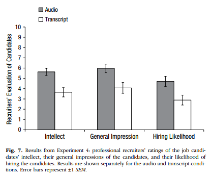
Figure 6.1: Figure 7 from Schroeder and Epley (2015) which you should try to replicate.

Replace the NULLs below to create a very basic version of this figure.

group_means <- group_by(ratings2, NULL, NULL) %>%
  summarise(Rating = mean(Rating))

ggplot(group_means, aes(NULL, NULL, fill = NULL)) +
  geom_col(position = "dodge")

Thinking Cap Point

Improve Your Figure: How could you improve this plot. What other geom_() options could you try? Are bar charts that informative or would something else be better? How would you add or change the labels of your plot? Could you change the colours in your figure?

Next, have a look at the possible solution below to see a modern way of presenting this information. There are some new functions in this solution that you should play about with to understand what they do. Remember it is a layering system, so remove lines and see what happens. Note how in the solution the Figure shows the raw data points as well as the means in each condition; this gives a better impression of the true data as just showing the means can be misleading. You can continue your further exploration of visualisations by reading this paper later when you have a chance: Weissberger et al., 2015, Beyond Bar and Line Graphs: Time for a New Data Presentation Paradigm

Filling in the code as below will create a basic figure as shown:

group_means <- ratings2 %>%
  group_by(condition, Category) %>%
  summarise(Rating = mean(Rating))

## `summarise()` has grouped output by 'condition'. You can override using the
## `.groups` argument.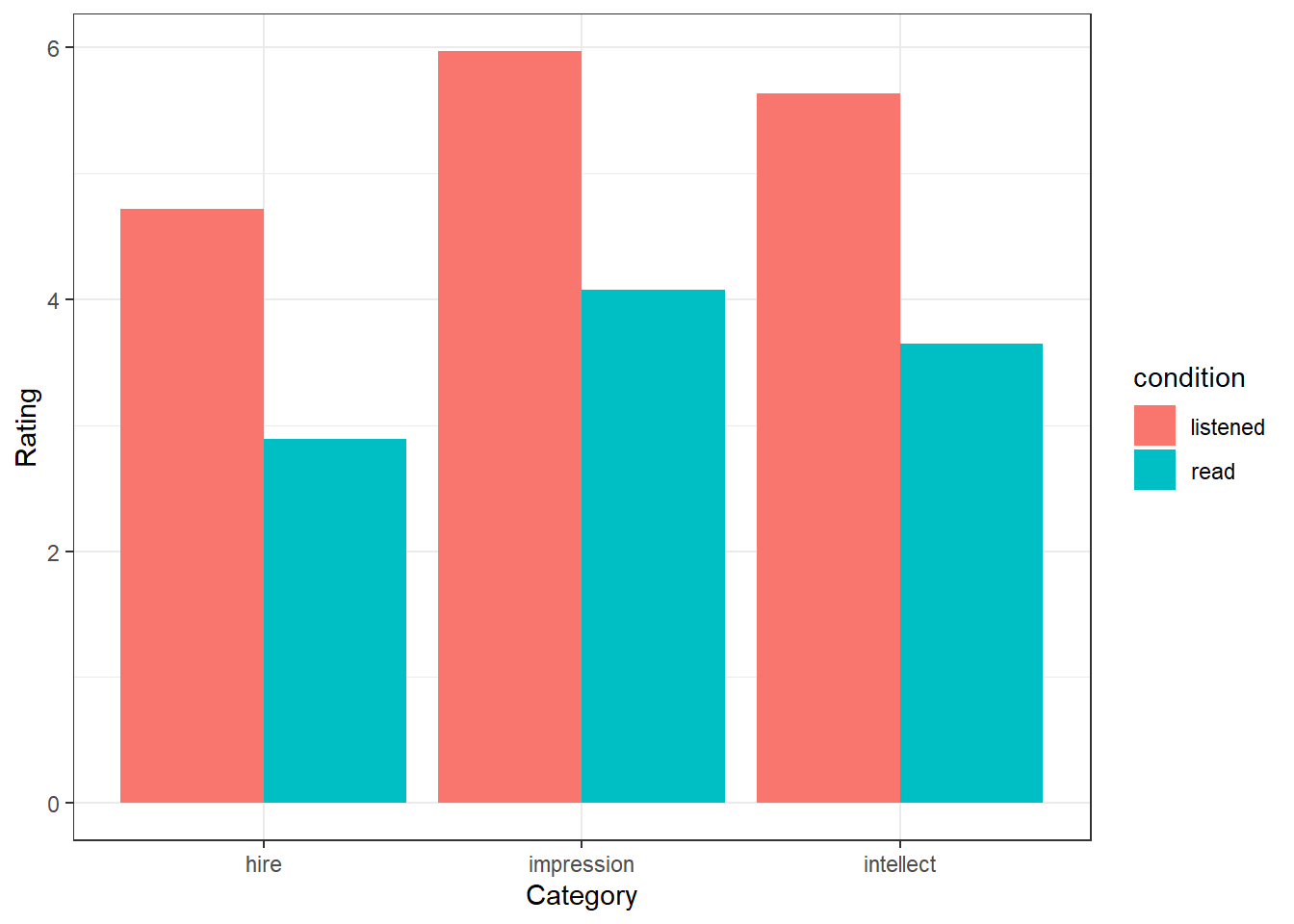

ggplot(group_means, aes(Category, Rating, fill = condition)) + 
  geom_col(position = "dodge")

Figure 6.2: A basic solution to Figure 7

Or alternatively, for a more modern presentation of the data:

group_means <- ratings2 %>%
  group_by(condition, Category) %>%
  summarise(Rating = mean(Rating))

## `summarise()` has grouped output by 'condition'. You can override using the
## `.groups` argument.

ggplot(ratings2, aes(condition, Rating, color = condition)) +
  geom_jitter(alpha = .4) +
  geom_violin(aes(fill = condition), alpha = .1) +
  facet_wrap(~Category) +
  geom_point(data = group_means, size = 2) +
  labs(x = "Category", y = "Recruiters' Evaluation of Candidates") +
  coord_cartesian(ylim = c(0, 10), expand = FALSE) +
  guides(color = "none", fill = "none") +
  theme_bw()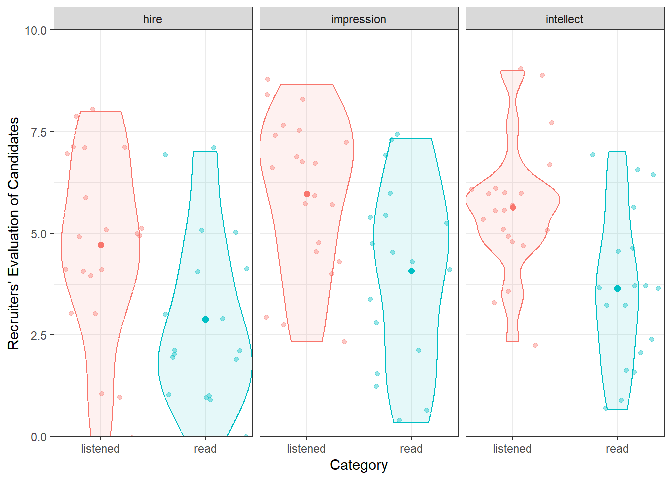

Figure 6.3: A possible alternative to Figure 7

6.3.4 Task 4: t-tests

Brilliant! So far we have checked the descriptives and the visualisations, and the last thing now is to check the inferential tests; the t-tests. You should still have ratings2 stored from Task 2. From this tibble, let's reproduce the t-test results from the article and at the same time show you how to run a t-test. You can refer back to the lectures to understand the maths of a between-subjects t-test, but essentially it is a measure between the difference in means over the variance about those means.

Here is a paragraph from the paper describing the results (p. 887):

"The pattern of evaluations by professional recruiters replicated the pattern observed in Experiments 1 through 3b (see Fig. 7). In particular, the recruiters believed that the job candidates had greater intellect---were more competent, thoughtful, and intelligent---when they listened to pitches (M = 5.63, SD = 1.61) than when they read pitches (M = 3.65, SD = 1.91), t(37) = 3.53, p < .01, 95% CI of the difference = [0.85, 3.13], d = 1.16. The recruiters also formed more positive impressions of the candidates---rated them as more likeable and had a more positive and less negative impression of them---when they listened to pitches (M = 5.97, SD = 1.92) than when they read pitches (M = 4.07, SD = 2.23), t(37) = 2.85, p < .01, 95% CI of the difference = [0.55, 3.24], d = 0.94. Finally, they also reported being more likely to hire the candidates when they listened to pitches (M = 4.71, SD = 2.26) than when they read the same pitches (M = 2.89, SD = 2.06), t(37) = 2.62, p < .01, 95% CI of the difference = [0.41, 3.24], d = 0.86."

We are going to run the t-tests for Intellect, Hire and Impression; each time comparing evaluators overall ratings for the listened group versus overall ratings for the read group to see if there was a significant difference between the two conditions: i.e., did the evaluators who listened to pitches give a significant higher or lower rating than evaluators that read pitches.

In terms of hypotheses, we could phrase the null hypothesis for these tests as there is no significant difference between overall ratings on the {insert trait} scale between evaluators who listened to resume pitches and evaluators who read the resume pitches (\(H_0: \mu_1 = \mu2\)). Alternatively, we could state it as there will be a significant difference between overall ratings on the {insert trait} scale between evaluators who listened to resume pitches and evaluators who read the resume pitches (\(H_1: \mu_1 \ne \mu2\)).

To clarify, we are going to run three between-subjects t-tests in total; one for intellect ratings; one for hire ratings; one for impression ratings. We will show you how to run the t-test on intellect ratings and then ask you to do the remaining two t-tests yourself.

To run this analysis on the intellect ratings you will need the function t.test() and you will use broom::tidy() to pull out the results from each t-test into a tibble. Below, we show you how to create the group means and then run the t-test for intellect. Run these lines and have a look at what they do.

First we calculate the group means:

group_means <- ratings2 %>%
  group_by(condition, Category) %>%
  summarise(m = mean(Rating), sd = sd(Rating))

## `summarise()` has grouped output by 'condition'. You can override using the
## `.groups` argument.

And we can call them and look at them by typing:

group_means

condition	Category	m	sd
listened	hire	4.714286	2.261479
listened	impression	5.968254	1.917477
listened	intellect	5.634921	1.608674
read	hire	2.888889	2.054805
read	impression	4.074074	2.233306
read	intellect	3.648148	1.911343

Now to just look at intellect ratings we need to filter them into a new tibble:

intellect <- filter(ratings2, Category == "intellect")

And then we run the actual t-test and tidy it into a table.
- t.test() requires two vectors as input
- pull() will pull out a single column from a tibble, e.g. Rating from intellect
- tidy() takes information from a test and turns it into a tibble. Try running the t.test with and without piping into tidy() to see what it does differently.

intellect_t <- t.test(intellect %>% 
                        filter(condition == "listened") %>% 
                        pull(Rating),
                      intellect %>% 
                        filter(condition == "read") %>% 
                        pull(Rating),
                      var.equal = TRUE) %>%
  tidy()

Now lets look at the intellect_ttibble we have created (assuming you piped into tidy()):

Table 6.1: The t-test output of those in the intellect condition.
estimate	estimate1	estimate2	statistic	p.value	parameter	conf.low	conf.high	method	alternative
1.987	5.635	3.648	3.526	0.001	37	0.845	3.128	Two Sample t-test	two.sided

From the tibble, intellect_t, you can see that you ran a Two Sample t-test (meaning between-subjects) with a two-tailed hypothesis test ("two.sided"). The mean for the listened condition, estimate1, was 5.635, whilst the mean for the read condition, estimate2 was 3.648 - compare these to the means in group_means as a sanity check. So overall there was a difference between the two means of 1.987. The degrees of freedom for the test, parameter, was 37. The observed t-value, statistic, was 3.526, and it was significant as the p-value, p.value, was p = 0.0011, which is lower than the field standard Type 1 error rate of \(\alpha = .05\).

As you will know from your lectures, a t-test is presented as t(df) = t-value, p = p-value. As such, this t-test would be written up as: t(37) = 3.526, p = 0.001.

Thinking about interpretation of this finding, as the effect was significant, we can reject the null hypothesis that there is no significant difference between mean ratings of those who listened to resumes and those who read the resumes, for intellect ratings. We can go further than that and say that the overall intellect ratings for those that listened to the resume was significantly higher (mean diff = 1.987) than those who read the resumes, t(37) = 3.526, p = 0.001, and as such we accept the alternative hypothesis. This would suggest that hearing people speak leads evaluators to rate the candidates as more intellectual than when you merely read the words they have written.

Now Try:

Running the remaining t-tests for hire and for impression. Store them in tibbles called hire_t and impress_t respectively.
Bind the rows of intellect_t, hire_t and impress_t to create a table of the three t-tests called results. It should look like this:

Table 6.2: Output of all three t-tests
Category	estimate	estimate1	estimate2	statistic	p.value	parameter	conf.low	conf.high	method	alternative
intellect	1.987	5.635	3.648	3.526	0.001	37	0.845	3.128	Two Sample t-test	two.sided
hire	1.825	4.714	2.889	2.620	0.013	37	0.414	3.237	Two Sample t-test	two.sided
impression	1.894	5.968	4.074	2.851	0.007	37	0.548	3.240	Two Sample t-test	two.sided

Quickfire Questions

Check your results for hire. Enter the mean estimates and t-test results (means and t-value to 2 decimal places, p-value to 3 decimal places):
- Mean estimate1 (listened condition) =
- Mean estimate2 (read condition) =
- t() = , p =
- Looking at this result, True or False, this result is significant at \(\alpha = .05\)?
Check your results for impression. Enter the mean estimates and t-test results (means and t-value to 2 decimal places, p-value to 3 decimal places):
- Meanestimate1 (listened condition) =
- Mean estimate2 (read condition) =
- t() = , p =
- Looking at this result, True or False, this result is significant at \(\alpha = .05\)?

Your t-test answers should have the following structure:

t(degrees of freedom) = t-value, p = p-value,

where:

degrees of freedom = parameter,
t-value = statistic,
and p-value = p.value.

Remember that if a result has a p-value lower (i.e. smaller) than or equal to the alpha level then it is said to be significant.

So to recap, we looked at the data from Schroeder and Epley (2015), both the descriptives and inferentials, we plotted a figure, and we confirmed that, as in the paper, there are significant differences in each of the three rating categories (hire, impression and intellect), with the listened condition receiving a higher rating than the read condition on each rating. All in, our interpretation would be that people rate you higher when they hear you speak your resume as opposed to them just reading your resume!

6.4 Student's versus Welch's t-tests

The between-subjects t-test comes in two versions: one assuming equal variance in the two groups (Student's t-test) and another not making this assumption (Welch's t-test). while the Student's t-test is considered the more common and standard t-test in the field, it is advisable to use the Welch's t-test instead.

The blog post "Always use Welch's t-test instead of Student's t-test" by Daniel Lakens shows that if the groups have equal variance then both tests return the same finding. However, if the assumption of equal variance is violated, i.e. the groups have unequal variance, then Welch's test produces the more accurate finding, based on the data.

This is important as often the final decision on whether assumptions are "held" or "violated" is subjective; i.e. it is down to the researcher to fully decide. Nearly all data will show some level of unequal variance (with perfectly equal variance across multiple conditions actually once revealing fraudulent data). Researchers using the Student's t-test regularly have to make a judgement about whether the variance across the two groups is "equal enough". As such, this blog shows that it is always better to run a Welch's t-test to analyse a between-subjects design as a) Welch's t-test does not have the assumption of equal variance, b) Welch's t-test gives more accurate results when variance is not equal, and c) Welch's t-test performs exactly the same as the Student t-test when variance is equal across groups.

In short, Welch's t-test takes a level of ambiguity (or what may be called a "researcher degree of freedom") out of the analysis and makes the analysis less open to bias or subjectivity. As such, from now on, unless stated otherwise, you should run a Welch's t-test.

In practice it is very easy to run the Welch's t-test, and you can switch between the tests as shown: * to run a Student's t-test you set var.equal = TRUE * to run a Welch's t-test you set var.equal = FALSE

This would run a Student's t-test:

t.test(my_dv ~ my_iv, data = my_data, var.equal = TRUE)

This would run the Welch's t-test:

t.test(my_dv ~ my_iv, data = my_data, var.equal = FALSE)

And two ways to know that you have run the Welch's t-test are:

The output says you ran the Welch Two Sample t-test
The df is likely to have decimal places in the Welch's t-test whereas it will be a whole number in the Student's t-test.

Always run the Welch's t-test in a between-subjects design when using R!

6.5 Practice Your Skills

6.5.1 Single-dose testosterone administration impairs cognitive reflection in men.

In order to complete this exercise, you first have to download the assignment .Rmd file which you need to edit for this assignment: titled GUID_Ch6_PracticeYourSkills.Rmd. This can be downloaded within a zip file from the link below. Once downloaded and unzipped you should create a new folder that you will use as your working directory; put the .Rmd file in that folder and set your working directory to that folder through the drop-down menus at the top. Download the Assignment .zip file from here.

For this assignment we will be using real data from the following paper:

Nave, G., Nadler, A., Zava, D., and Camerer, C. (2017). Single-dose testosterone administration impairs cognitive reflection in men. Psychological Science, 28, 1398--1407.

The full data documentation can be found on the Open Science Framework repository, but for this assignment we will just use the .csv file in the zipped folder: CRT_Data.csv. You may also want to read the paper, at least in part, to help fully understand this analysis if at times you are unsure. Here is the article's abstract:

In nonhumans, the sex steroid testosterone regulates reproductive behaviors such as fighting between males and mating. In humans, correlational studies have linked testosterone with aggression and disorders associated with poor impulse control, but the neuropsychological processes at work are poorly understood. Building on a dual-process framework, we propose a mechanism underlying testosterone's behavioral effects in humans: reduction in cognitive reflection. In the largest study of behavioral effects of testosterone administration to date, 243 men received either testosterone or placebo and took the Cognitive Reflection Test (CRT), which estimates the capacity to override incorrect intuitive judgments with deliberate correct responses. Testosterone administration reduced CRT scores. The effect remained after we controlled for age, mood, math skills, whether participants believed they had received the placebo or testosterone, and the effects of 14 additional hormones, and it held for each of the CRT questions in isolation. Our findings suggest a mechanism underlying testosterone's diverse effects on humans' judgments and decision making and provide novel, clear, and testable predictions.

The critical findings are presented on p. 1403 of the paper under the heading "The influence of testosterone on CRT performance". Your task today is to attempt to try and reproduce some of the main results from the paper.

Note: Being unable to get the exact same results as the authors doesn't necessarily mean you are wrong! The authors might be wrong, or might have left out important details. Present what you find.

Before starting lets check:

The .csv file is saved into a folder on your computer and you have manually set this folder as your working directory.
The .Rmd file is saved in the same folder as the .csv files. For assessments we ask that you save it with the format GUID_Ch6_PracticeYourSkills.Rmd where GUID is replaced with your GUID. Though this is a formative assessment, it may be good practice to do the same here.

6.5.2 Task 1A: Libraries

In today's exercise you will need both the tidyverse and broom packages. Enter code into the t1A code chunk below to load in both of these libraries.

## load in the tidyverse and broom packages

6.5.3 Task 1B: Loading in the data

Use read_csv() to replace the NULL in the t1B code chunk below to load in the data stored in the data file CRT_Data.csv. Store the data in the variable crt. Do not change the file name of the data file.

crt <- NULL

6.5.4 Task 2: Selecting only relevant columns

Have a look at crt. There are three variables in crt that you will need to find and extract in order to perform the t-test: the subject ID number (hint: each participant has a unique number); the independent variable (hint: each participant has the possibility of being in one of two treatments coded as 1 or 0); and the dependent variable (hint: the test specifically looks at which answers people get correct). Identify those three variables. It might help to look at the first few sentences under the heading "The influence of testosterone on CRT performance" and Figure 2a in the paper for further guidance on the correct variables.

Having identified the important three columns, replace the NULL in the t2 code chunk below to select out only those three columns from crt and store them in the tibble crt2.

Check your work: If correct, crt2 should be a tibble with 3 columns and 243 rows.

crt2 <- NULL

Note: For the remainder of this assignment you should use crt2 as the main source tibble and not crt.

6.5.5 Task 3: Verify the number of subjects in each group

The Participants section of the article contains the following statement:

243 men (mostly college students; for demographic details, see Table S1 in the Supplemental Material available online) were randomly administered a topical gel containing either testosterone (n = 125) or placebo (n = 118).

In the t3 code block below, replace the NULLs with lines of code to calculate:

The number of men in each Treatment. This should be a tibble called cond_counts containing a column called Treatment showing the two groups and a column called n which shows the number of men in each group.
The total number of men in the sample. This should be a single value, not a tibble, and should be stored in n_men.

You know the answer to both of these tasks already. Make sure that your code gives the correct answer!

cond_counts <- NULL
n_men <- NULL

Now replace the strings in the statements below, using inline R code, so that it reproduces the sentence from the paper exactly as it is shown above. In other words, in the statement below, anywhere it says "(your code here)", replace that string (including the quotes), with inline R code. To clarify, when looking at the .Rmd file you should see R code, but when looking at the knitted file, you should see values. Look back at Chapter 1 if you are unsure of how to use inline code.

Hint: One solution is to do something with cond_counts similar to what we did with filter() and pull() in the exercises of this Chapter.

"(your code here)" men (mostly college students; for demographic details, see Table S1 in the Supplemental Material available online) were randomly administered a topical gel containing either testosterone (n = "(your code here)") or placebo (n = "(your code here)").

6.5.6 Task 4: Reproduce Figure 2a

Here is Figure 2A from the original paper:

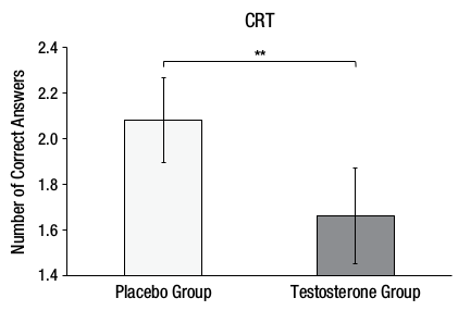
Figure 6.4: Figure 2A from Nave, Nadler, Zava, and Camerer (2017) which you should replicate

Write code in the t4 code chunk to reproduce a version of Figure 2a - shown above. Before you create the plot, replace the NULL to make a tibble called crt_means with the mean and standard deviation of the number of CorrectAnswers for each group.
Use crt_means as the source data for the plot.

Hint: you will need to check out recode() to get the labels of treatments right. Look back at Chapter 2 for a hint on how to use recode(). Or check this short resource for examples on how to use recode(): Recode short tutorial.

Don't worry about including the error bars (unless you want to) or the line indicating significance in the plot. Do however make sure to pay attention to the labels of treatments and of the y-axis scale and label. Reposition the x-axis label to below the Figure. You can use colour, if you like.

crt_means <- NULL

## TODO: add lines of code using ggplot

6.5.7 Task 5: Interpreting your Figure

Always good to do a slight recap at this point to make sure you are following the analysis. Replace the NULL in the t5 code chunk below with the number of the statement that best describes the data you have calculated and plotted thus far. Store this single value in answer_t5:

The Testosterone group (M = 2.10, SD = 1.02) would appear to have fewer correct answers on average than the Placebo group (M = 1.66, SD = 1.18) on the Cognitive Reflection Test suggesting that testosterone does in fact inhibit the ability to override incorrect intuitive judgments with the correct response.
The Testosterone group (M = 1.66, SD = 1.18) would appear to have more correct answers on average than the Placebo group (M = 2.10, SD = 1.02) on the Cognitive Reflection Test suggesting that testosterone does in fact inhibit the ability to override incorrect intuitive judgments with the correct response.
The Testosterone group (M = 1.66, SD = 1.18) would appear to have fewer correct answers on average than the Placebo group (M = 2.10, SD = 1.02) on the Cognitive Reflection Test suggesting that testosterone does in fact inhibit the ability to override incorrect intuitive judgments with the correct response.
The Testosterone group (M = 2.10, SD = 1.02) would appear to have more correct answers on average than the Placebo group (M = 1.66, SD = 1.18) on the Cognitive Reflection Test suggesting that testosterone does in fact inhibit the ability to override incorrect intuitive judgments with the correct response.

answer_t5 <- NULL

6.5.8 Task 6: t-test

Now that we have calculated the descriptives in our study we need to run the inferentials. In the t6 code chunk below, replace the NULL with a line of code to run the t-test taking care to make sure that the output table has the Placebo mean under Estimate1 (group 0) and Testosterone mean under Estimate2 (group 1). Assume variance is equal and use broom::tidy() to sweep and store the results into a tibble called t_table.

t_table <- NULL

6.5.9 Task 7: Reporting results

In the t7A code chunk below, replace the NULL with a line of code to pull out the df from t_table. This must be a single value stored in t_df.

t_df <- NULL

In the t7B code chunk below, replace the NULL with a line of code to pull out the t-value from t_table. Round it to three decimal places. This must be a single value stored in t_value.

t_value <- NULL

In the t7C code chunk below, replace the NULL with a line of code to pull out the p-value from t_table. Round it to three decimal places. This must be a single value stored in p_value.

p_value <- NULL

In the t7D code chunk below, replace the NULL with a line of code to calculate the absolute difference between the mean number of correct answers for the Testosterone group and the Placebo group. Round it to three decimal places. This must be a single value stored in t_diff.

t_diff <- NULL

If you have completed t7A to t7D accurately, then when knitted, one of these statements below will produce an accurate and coherent summary of the results. In the t7E code chunk below, replace the NULL with the number of the statement below that best summarises the data in this study. Store this single value in answer_t7e

The testosterone group performed significantly better ( fewer correct answers) than the placebo group, t() = , p = .
The testosterone group performed significantly worse ( fewer correct answers) than the placebo group, t() = , p = .
The testosterone group performed significantly better ( more correct answers) than the placebo group, t() = , p = .
The testosterone group performed significantly worse ( fewer correct answers) than the placebo group, t() = , p = .

answer_t7e <- NULL

Well done, you are finished! Now you should go check your answers against the solutions at the end of this chapter. You are looking to check that the resulting output from the answers that you have submitted are exactly the same as the output in the solution - for example, remember that a single value is not the same as a coded answer. Where there are alternative answers, it means that you could have submitted any one of the options as they should all return the same answer.

6.6 Solutions to Questions

6.6.1 The Two-Sample t-test

6.6.1.1 Task 1

library("tidyverse")
library("broom") # you'll need broom::tidy() later

evaluators <- read_csv("evaluators.csv")

evaluators %>%
  summarize(mean_age = mean(age, na.rm = TRUE))

evaluators %>%
  count(sex)

# If using `recode()`:
evaluators %>%
  count(sex) %>%
  mutate(sex_names = recode(sex, "1" = "male", "2" = "female"))

The mean age of the evaluators was 30.9
The standard deviatoin of the age of the evaluators was 6.24
There were 4 males and e_count %>% filter(sex_names == "female") %>% pull(n) females, with 5 people not stating a sex.

Return to Task

6.6.1.2 Task 2

load in the data

ratings <- read_csv("ratings.csv")

First pull out the ratings associated with intellect

iratings <- ratings %>%
  filter(Category %in% c("competent", "thoughtful", "intelligent"))

Next calculate means for each evaluator

imeans <- iratings %>%
  group_by(eval_id) %>%
  summarise(Rating = mean(Rating))

Mutate on the Category variable. This way we can combine with 'impression' and 'hire' into a single table which will be very useful!

imeans2 <- imeans %>%
  mutate(Category = "intellect")

And then combine all the information in to one single tibble.

ratings2 <- ratings %>%
  filter(Category %in% c("impression", "hire")) %>%
  bind_rows(imeans2) %>%
  inner_join(evaluators, "eval_id") %>%
  select(-age, -sex) %>%
  arrange(eval_id, Category)

Return to Task

6.6.1.3 Task 4

First we calculate the group means:

group_means <- ratings2 %>%
  group_by(condition, Category) %>%
  summarise(m = mean(Rating), sd = sd(Rating))

## `summarise()` has grouped output by 'condition'. You can override using the
## `.groups` argument.

And we can call them and look at them by typing:

group_means

Now to just look at intellect ratings we need to filter them into a new tibble:

intellect <- filter(ratings2, Category == "intellect")

And then we run the actual t-test and tidy it into a table.
- t.test() requires two vectors as input
- pull() will pull out a single column from a tibble, e.g. Rating from intellect
- tidy() takes information from a test and turns it into a table. Try running the t.test with and without piping into tidy() to see what it does differently.

intellect_t <- t.test(intellect %>% filter(condition == "listened") %>% pull(Rating),
                      intellect %>% filter(condition == "read") %>% pull(Rating),
                      var.equal = TRUE) %>%
  tidy()

Now we repeat for HIRE and IMPRESSION

hire <- filter(ratings2, Category == "hire")
hire_t <- t.test(hire %>% filter(condition == "listened") %>% pull(Rating),
                      hire %>% filter(condition == "read") %>% pull(Rating),
                 var.equal = TRUE) %>%
  tidy()

And for Impression

impress <- filter(ratings2, Category == "impression")
impress_t <- t.test(impress %>% filter(condition == "listened") %>% pull(Rating),
                    impress %>% filter(condition == "read") %>% pull(Rating),
                    var.equal = TRUE) %>%
  tidy()

Before combining all into one table showing all three t-tests

results <- bind_rows("hire" = hire_t, 
                     "impression" = impress_t,
                     "intellect" = intellect_t, .id = "id")

results

Return to Task

6.6.2 Practice Your Skills

6.6.2.1 Task 1A: Libraries

library(broom)
library(tidyverse)

Return to Task

6.6.2.2 Task 1B: Loading in the data

Use read_csv() to read in data!

crt <- read_csv("data/06-s01/homework/CRT_Data.csv")

crt <- read_csv("CRT_Data.csv")

Return to Task

6.6.2.3 Task 2: Selecting only relevant columns

The key columns are:

ID
Treatment
CorrectAnswers

Creating crt2 which is a tibble with 3 columns and 243 rows.

crt2 <- select(crt, ID, Treatment, CorrectAnswers)

Return to Task

6.6.2.4 Task 3: Verify the number of subjects in each group

The Participants section of the article contains the following statement:

In the t3 code block below, replace the NULLs with lines of code to calculate:

The number of men in each Treatment. This should be a tibble/table called cond_counts containing a column called Treatment showing the two groups and a column called n which shows the number of men in each group.
The total number of men in the sample. This should be a single value, not a tibble/table, and should be stored in n_men.

You know the answer to both of these tasks already. Make sure that your code gives the correct answer!

For cond_counts, you could do:

cond_counts <- crt2 %>% group_by(Treatment) %>% summarise(n = n())

Or alternatively

cond_counts <- crt2 %>% count(Treatment)

For n_men, you could do:

n_men <- crt2 %>% summarise(n = n()) %>% pull(n)

Or alternatively

n_men <- nrow(crt2)

Solution:

When formatted with inline R code as below:

`r n_men` men (mostly college students; for demographic details, see Table S1 in the Supplemental Material available online) were randomly administered a topical gel containing either testosterone (n = `r cond_counts %>% filter(Treatment == 1) %>% pull(n)`) or placebo (n = `r cond_counts %>% filter(Treatment == 0) %>% pull(n)`).

should give:

Return to Task

6.6.2.5 Task 4: Reproduce Figure 2A

You could produce a good representation of Figure 2A with the following approach:

crt_means <- crt2 %>% 
  group_by(Treatment) %>% 
  summarise(m = mean(CorrectAnswers), sd = sd(CorrectAnswers)) %>%
  mutate(Treatment = recode(Treatment, "0" = "Placebo", "1" = "Testosterone Group"))

ggplot(crt_means, aes(Treatment, m, fill = Treatment)) + 
  geom_col() + 
  theme_classic() + 
  labs(x = "CRT", y = "Number of Correct Answers") +
  guides(fill = "none") +
  scale_fill_manual(values = c("#EEEEEE","#AAAAAA")) +
  coord_cartesian(ylim = c(1.4,2.4), expand = TRUE)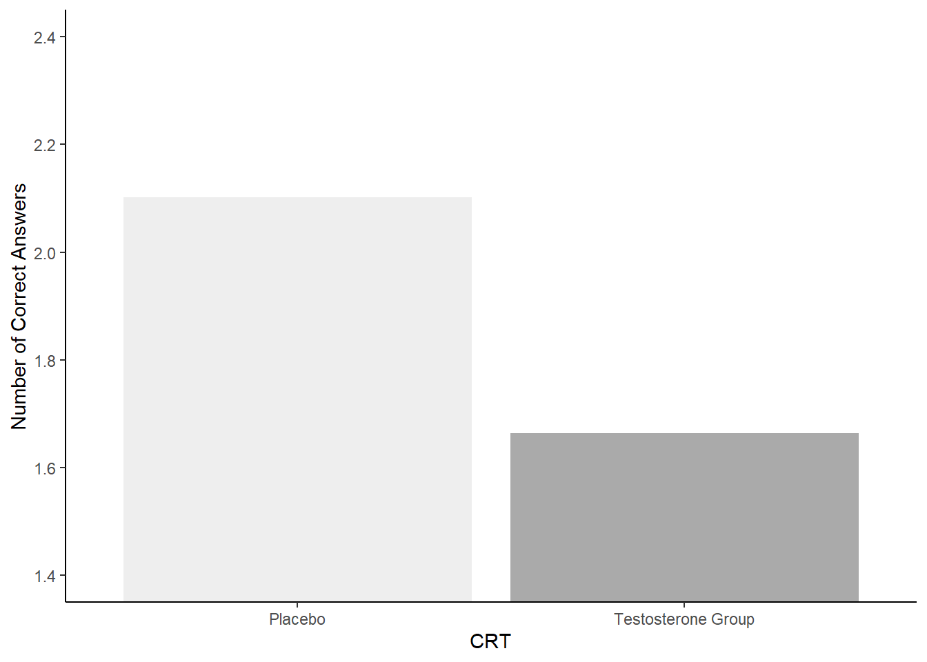

Figure 6.5: A representation of Figure 2A

Return to Task

6.6.2.6 Task 5: Interpreting your Figure

Option 3 is the correct answer given that:

The Testosterone group (M = 1.66, SD = 1.18) would appear to have fewer correct answers on average than the Placebo group (M = 2.10, SD = 1.02) on the Cognitive Reflection Test suggesting that testosterone does in fact inhibit the ability to override incorrect intuitive judgements with the correct response.

answer_t5 <- 3

Return to Task

6.6.2.7 Task 6: t-test

You need to pay attention to the order when using this first approach, making sure that the 0 group are entered first. This will put the Placebo groups as Estimate1 in the output. In reality it does not change the values, but the key thing is that if you were to pass this code on to someone, and they expect Placebo to be Estimate1, then you need to make sure you coded it that way.

t_table <- t.test(crt2 %>% filter(Treatment == 0) %>% pull(CorrectAnswers),
                  crt2 %>% filter(Treatment == 1) %>% pull(CorrectAnswers),
                  var.equal = TRUE) %>%
  tidy()

Alternatively, you could use what is known as the formula approach as shown below. Here you state the DV ~ IV and you say the name of the tibble in data = .... You just need to make sure that the columns you state as the DV and the IV are actually in the tibble!

t_table <- t.test(CorrectAnswers ~ Treatment, data = crt2, var.equal = TRUE) %>% tidy()

Note that this approach will compare based on the alphabetical or numerical order of the values in the independent variable. Therefore, the 0 group would still be the first group in the comparison, matching the previous approach.

Return to Task

6.6.2.8 Task 7: Reporting results

The degrees of freedom (df) is found under parameter

t_df <- t_table$parameter

An alternative option for this would be as follows, using the pull() method. This would work for B to D as well

t_df <- t_table %>% pull(parameter)

The t-value is found under statistic

t_value <- t_table$statistic %>% round(3)

The p-value is found under p.value

p_value <- t_table$p.value %>% round(3)

The absolute difference between the two means can be calculated as follows:

t_diff <- (t_table$estimate1 - t_table$estimate2) %>% round(3) %>% abs()

If you have completed t7A to t7D accurately, then when knitted, Option 4 would be stated as such

The testosterone group performed significantly worse (0.438 fewer correct answers) than the placebo group, t(241) = 3.074, p = 0.002

and would therefore be the correct answer!

answer_t7e <- 4

Return to Task

Chapter Complete!

5 NHST: Binomial test and One-Sample t-test

7 NHST: Paired-Sample t-test and Nonparametric tests