5  Logistic Regression

Attaching package: 'glossary'

The following object is masked from 'package:webexercises':

    add_to_quarto

In this chapter, we build on simple and multiple linear regression. All the lessons you learnt there still apply for building models with one or more predictors, but sometimes it is not appropriate to assume normality. It is a popular and convenient choice as assuming normality is often robust, but for some outcomes it would simply not be the appropriate choice. Generalised linear models allow you to specify a link and link function for the model residuals, so you can apply a linear model to alternative distributions. In this chapter, we will cover logistic regression for modeling dichotomous outcomes.

Chapter Intended Learning Outcomes (ILOs)

By the end of this chapter, you should be able to:

• Understand how to run and interpret logistic regression.

5.1 Chapter preparation

5.1.1 Organising your files and project for the chapter

Before we can get started, you need to organise your files and project for the chapter, so your working directory is in order.

1. In your folder for statistics and research design Stats_Research_Design, create a new folder called 05_regression_generalised. Within 05_logistic, create two new folders called data and figures.

2. Create an R Project for 05_logistic as an existing directory for your chapter folder. This should now be your working directory.

3. Create a new Quarto document and give it a sensible title describing the chapter, such as 05 Logistic Regression. Save the file in your 05_logistic folder.

4. We are working with a few data sets in this chapter, so please save the following zip file containing all the data files you need: Chapter 05 Data. Right click the link and select “save link as”, or clicking the link will save the file to your Downloads. Extract the files and make sure that you save them as “.csv”. Save or copy the files to your data/ folder within 05_logistic.

You are now ready to start working on the chapter!

5.2 Logistic Regression

5.2.1 Introduction to the dataset

For the guided examples, we have two datasets, but we will introduce them in turn. To demonstrate logistic regression, we will use data from Bostyn et al. (2018).

Bostyn et al. studied the classic trolley-dilemma in moral philosophy. In the typical format, a trolley (streetcar/tram) is travelling along tracks and will run over five people. However, you have the choice to pull a lever and divert the trolley to run over just one person. Although this would save lives, you must manually intervene to essentially kill one person. This is typically always a hypothetical scenario as it’s difficult to ask an ethics board for permission to run over people. In this study, Bostyn et al. compared a hypothetical version of the trolley-dilemma with a (seemingly) realistic version. Participants chose between not intervening and allowing five mice in a cage to be shocked with electricity or they could intervene and one mouse would be shocked instead. Do not worry, the mice were never shocked but participants did not know it at the time.

Their research question was: would there be a difference in moral decision-making when participants completed a hypothetical compared to a real version of the trolley-dilemma task? There was seemingly no hypothesis, so we will just focus on addressing the research question.

There is one independent variable (STUDY) to randomly allocate participants into one of two groups:

1. The “real” group (group 1 in the data) attended a lab session where they saw two cages of real mice. They had 20 seconds to decide whether to press a button and divert the electric shock to the cage with one mouse.

2. The hypothetical group (group 2 in the data) completed a more traditional version of the study where they just responded on a computer for whether they would intervene or not after reading a description of allowing five mice to be shocked or choosing for one mouse to be shocked.

Participants completed a bunch of additional measures on moral judgement, empathy, psychopathy etc., but our main outcome of interest is whether they chose to intervene (1) or not (0) from the variable DECISION. They label these two decisions as deontological when people intervened and consequentialist when people did not intervene. For plotting, we will use the labels, but for the analyses we will use the 0s and 1s.

We first need to load some packages and the data for this task. If you do not have any of the packages, make sure you install them first.

As the first activity, try and test yourself by completing the following task list to practice your data wrangling skills. Create a final object called bostyn_data to be consistent with the tasks below. If you just want to focus on fitting the models, then you can just copy the code in the solution.

TipTry this

To wrangle the data, complete the following tasks:

1. Load the following packages. If you do not have them already, remember you will need to install them first if you are working on your own computer:

   • tidyverse

   • emmeans

   • ordinal

   • sjPlot

2. You can complete the following tasks individually or combining things in one pipe, you just need a final object called bostyn_data. Read the data file data/bostyn_2018.csv.

3. There are loads of variables in the data which you can explore in your own time, but for this chapter, just select the first four variables from STUDY to DECISION.

4. There are a few missing values in DECISION, so remove the NAs at this point.

5. To help with plotting and modelling later, create two new variables:

   • Create a new variable called study where you create a factor to recode the values from STUDY. 1 should be relabelled “Real” and 2 should be relabelled as “Hypothetical”.

   • Create a new variable called label where you create a factor to recode the values from DECISION. 0 should be relabelled “DEO” for deontological and 1 should be relabelled as “CON” for consequentialist.

6. To help with modelling later, convert GENDER to a factor.

CautionShow me the solution

You should have the following in a code chunk:

# wrangling and visualisation functions 
library(tidyverse)
# Parameter estimates
library(emmeans)
# Ordinal regression for later
library(ordinal)
# plotting model objects
library(sjPlot)

# Bostyn data for logistic regression
bostyn_data <-read_csv("data/Bostyn_2018.csv") %>% 
  select(STUDY:DECISION) %>%  # just select first four variables
  drop_na(DECISION) %>% 
  mutate(study = factor(STUDY, 
                        levels = c(1, 2), 
                        labels = c("Real", "Hypothetical")),
         label = factor(DECISION, 
                           levels = c(0, 1), 
                           labels = c("DEO", "CON")),
         GENDER = as.factor(GENDER))

5.2.2 Exploratory data analysis

When starting any data analysis, it is important to visualise the data for some exploratory data analysis. Using the skills you developed in data skills for reproducible research, you can explore the data to understand its properties and look for potential patterns. In this scenario, a bar plot might be handy as we have a dichotomous outcome, so we can explore the frequency of responses across each group.

bostyn_data %>% 
  ggplot(aes(x = study, fill = label)) + 
  geom_bar(position = "dodge") + 
  scale_x_discrete(name = "Study") + 
  scale_y_continuous(name = "Frequency", 
                     breaks = seq(0, 200, 50), 
                     limits = c(0,200)) + 
  scale_fill_viridis_d(name = "Decision", option = "E") +
  theme_minimal()

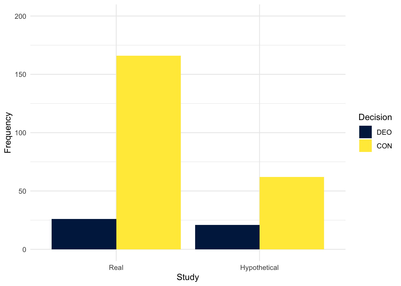
In the real group, there is a bigger difference in the number of people choosing to intervene and make a consequentialist response (1s in the data) compared to the hypothetical group where there is a smaller difference. The number of people choosing not to intervene and make a deontological response (0s in the data) is smaller in both groups, but it’s the proportional difference which changes.

Instead of counts, we can also express binary 0 and 1 data as a proportion or probability of intervening. If you take the mean of binary data, it tells you the proportion, so we can calculate the proportion of participant’s choosing to intervene as a consequentialist decision.

bostyn_data %>% 
  group_by(study) %>% 
  summarise(proportion_con = mean(DECISION))

study	proportion_con
Real	0.8645833
Hypothetical	0.7469880

Participants in the real group (86%) were more likely to intervene than participants in the hypothetical group (75%). These are just descriptive statistics though, so you need to think about modelling to make inferences from these data.

5.2.3 Would linear regression work?

Warning

The most important part of data analysis is your role as the decision maker and thinking about what would be the most appropriate choice of model. Sometimes, there are equally valid approaches, while other times there is one better suited approach. If you apply an inappropriate test, R will gladly follow your instructions. Its your job to think critically about your modelling approach and check its an appropriate choice.

When we have a dichotomous outcome coded 0 and 1, it has numerical value, so R will happily apply regular linear regression.

bostyn_model1 <- lm(DECISION ~ study, data = bostyn_data)

summary(bostyn_model1)

Call:
lm(formula = DECISION ~ study, data = bostyn_data)

Residuals:
    Min      1Q  Median      3Q     Max 
-0.8646  0.1354  0.1354  0.1354  0.2530 

Coefficients:
                  Estimate Std. Error t value Pr(>|t|)    
(Intercept)        0.86458    0.02698  32.041   <2e-16 ***
studyHypothetical -0.11760    0.04912  -2.394   0.0173 *  
---
Signif. codes:  0 '***' 0.001 '**' 0.01 '*' 0.05 '.' 0.1 ' ' 1

Residual standard error: 0.3739 on 273 degrees of freedom
Multiple R-squared:  0.02056,   Adjusted R-squared:  0.01698 
F-statistic: 5.732 on 1 and 273 DF,  p-value: 0.01733

It is somewhat interpretable as when you take the mean of binary data, you get the proportion. So, the intercept represents the proportion of consequentialist responses for those in the real group, and the slope coefficient represents the mean difference in proportion, suggesting there are .12/12% fewer consequentialist responses in the hypothetical group, which is statistically significant at \(\alpha\) = .05.

Although it works and we can make sense of the results, the question is whether it is an informative and appropriate way of modelling a binary outcome. Lets check the assumptions to see if anything looks off.

# Change the panel layout to 2 x 2
par(mfrow=c(2,2))

# plot the diagnostic plots
plot(bostyn_model1)

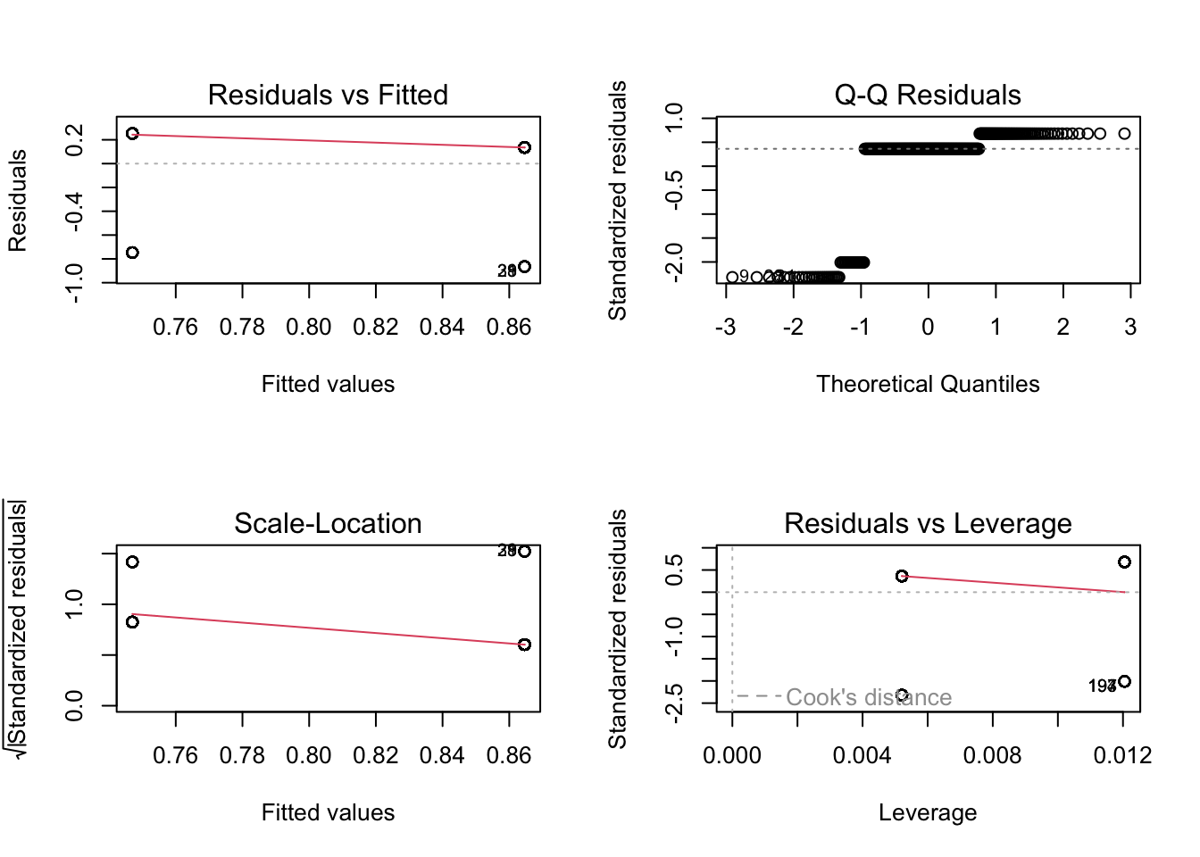
Now we can see the problems. Because we only have two possible outcomes, the assumption checks are all off. The qq plot in panel 2 particularly shows the problem, as there is a giant chunk missing where the values between 0 and 1 should be, at least theoretically if we assume normal residuals.

# plot the qq plot
plot(bostyn_model1, 
     which = 2)

Now we can apply logistic regression to more appropriately model the dichotomous nature of the outcome.

5.2.4 Logistic regression

5.2.4.1 Generalised linear regression

In a linear model, we model the outcome as a product of an intercept, a slope, and error. Its that final error part which is why we have worried about normality so far. In a regular linear regression model, we need the model residuals (the difference between the expected and observed values) to be normally distributed.

Logistic regression is an adaptation of the linear regression framework we have worked with so far, where we can replace that error component. This is called generalised linear regression and we can specify a link and link function, instead of normal residuals being built into the model.

So far, we have always used lm(), but R comes with another function called glm() for generalised linear regression models. To demonstrate how we can set the link family, we can use it to recreate a regular linear regression model, but this time explicitly calling a normal distribution as the link (using its alternate name a Gaussian distribution) and “identity” as the link function.

bostyn_model1_glm <- glm(DECISION ~ study, 
                     family = gaussian(link = "identity"), 
                     data = bostyn_data)

summary(bostyn_model1_glm)

Call:
glm(formula = DECISION ~ study, family = gaussian(link = "identity"), 
    data = bostyn_data)

Coefficients:
                  Estimate Std. Error t value Pr(>|t|)    
(Intercept)        0.86458    0.02698  32.041   <2e-16 ***
studyHypothetical -0.11760    0.04912  -2.394   0.0173 *  
---
Signif. codes:  0 '***' 0.001 '**' 0.01 '*' 0.05 '.' 0.1 ' ' 1

(Dispersion parameter for gaussian family taken to be 0.1398019)

    Null deviance: 38.967  on 274  degrees of freedom
Residual deviance: 38.166  on 273  degrees of freedom
AIC: 243.34

Number of Fisher Scoring iterations: 2

The link specifies the distribution family and the link function is the transformation for the model units. So, for our normal/Gaussian distribution, we have an identity link which essentially means no transformation, just the values we input. A normal distribution is described by a mean and standard deviation, so we just interpret the raw units in the model.

The results here are the same to the third decimal to show its an identical process. The only difference to our regular model output is the model fit statistics. Regular linear regression uses ordinal least squares to fit the model, whereas generalised linear regression fits the models using maximum likelihood. Holding everything else constant, this requires greater computing power, so its overkill to use glm() when you just want to assume normal/Gaussian errors, but its important to show the process behind these procedures.

Note

In this chapter, we are focusing on logistic regression and ordinal regression as variations of generalised linear regression. There are more possibilities though, so type ?family into the console to see the different families you could enter for the link and link function.

5.2.4.2 Logistic regression in glm()

After that brief detour, we will now actually fit the logistic regression model using glm(). As we have a dichotomous outcome, one useful distribution is the binomial. This applies when you want to calculate the probability of an dichotomous outcome from a series of successes (1s) and failures (0s). This models that probability nicely as it has a boundary of 0 or 0% (no successes) and 1 or 100% (all successes). Traditionally, we refer to successes and failures, but you can apply it to any binary outcome where one response is labelled 0 and the other response is labelled 1.

To apply the linear model element, we then use the “logit” link function as the unit transformation. Probability ranges between 0 and 1, odds range between 0 and infinity, but log odds (the logit bit) range between minus infinity and infinity, meaning we can fit straight lines to it. Let’s see what a logistic regression model looks like.

bostyn_model2 <- glm(DECISION ~ study, 
                     family = binomial(link = "logit"), 
                     data = bostyn_data)

summary(bostyn_model2)

Call:
glm(formula = DECISION ~ study, family = binomial(link = "logit"), 
    data = bostyn_data)

Coefficients:
                  Estimate Std. Error z value Pr(>|z|)    
(Intercept)         1.8539     0.2109   8.790   <2e-16 ***
studyHypothetical  -0.7713     0.3290  -2.344   0.0191 *  
---
Signif. codes:  0 '***' 0.001 '**' 0.01 '*' 0.05 '.' 0.1 ' ' 1

(Dispersion parameter for binomial family taken to be 1)

    Null deviance: 251.53  on 274  degrees of freedom
Residual deviance: 246.17  on 273  degrees of freedom
AIC: 250.17

Number of Fisher Scoring iterations: 4

confint(bostyn_model2)

Waiting for profiling to be done...

                     2.5 %    97.5 %
(Intercept)        1.45962  2.289875
studyHypothetical -1.41563 -0.120060

The model looks reassuringly similar. We have our coefficients for the intercept and slope, with their standard errors and p-values. There are no p-values for the model fit though as remember they are based on maximum likelihood, rather than least squares.

The main difference here is the interpretation of the coefficients. The link function is logit, so we get them in log odds, meaning the logarithm of an odds ratio (how likely something is to happen). These are not intuitive to interpret, so we can take the exponential to transform the slope coefficient from log odds to an odds ratio with its 95% CI.

# Take the exponential of the second coefficient to avoid typing it manually
exp(coef(bostyn_model2)[2]) #subset second component

studyHypothetical 
        0.4624211 

# Exponential of the confidence interval
exp(confint(bostyn_model2))

Waiting for profiling to be done...

                      2.5 %    97.5 %
(Intercept)       4.3043235 9.8737011
studyHypothetical 0.2427726 0.8868672

An odds ratio is a ratio of the odds of an event happening in one group compared to the odds of an event happening in another group. In this context, a ratio of making a consequentialist decision (1s compared to 0s) in the real group compared to the hypothetical group.

An odds ratio of 1 means they are equally likely to happen. An odds ratio of less than 1 means something is less likely to happen, whereas more than 1 means something is more likely to happen. The odds ratio is 0.46 here, suggesting the odds of making a consequentialist decision is lower in the hypothetical group (our target group) compared to the real group (the reference group). Odds ratios below 1 can be tricky to interpret, so you can flip them around by taking the reciprocal.

# Take the reciprocal of the exponential of the second coefficient 
1 / exp(coef(bostyn_model2)[2])

studyHypothetical 
         2.162531 

# Reciprocal of the exponential of the confidence interval
1 / exp(confint(bostyn_model2))

Waiting for profiling to be done...

                      2.5 %    97.5 %
(Intercept)       0.2323245 0.1012791
studyHypothetical 4.1190801 1.1275645

Expressed this way, there are 2.16 (95% CI = [1.13, 4.12]) lower odds of making a consequentialist decision in the hypothetical group compared to the real group. In this model, it is statistically significant but we can see there is a decent amount of uncertainty around the estimate, spanning from 1.13 to 4.12.

Important

In this scenario, you would get the same reciprocal odds ratio if you changed the groups around with correction as the reference group. Taking the reciprocal is the same information expressed differently, but its important you are clear about the model estimates to avoid confusing your reader. If you do this yourself, make sure you explain what the model estimates were and how you took the reciprocal.

5.2.4.3 Calculating the model probability estimates

Finally, there is a relationship between probability, odds, and log odds. We can use the coefficients to produce model estimates for the probability of a consequentialist decision in each group. Voas & Watt (2024) recommend this as the key output of a logistic regression model for helping to communicate your findings.

Warning

Relatedly, the whole purpose of Voas & Watt (2024) is to warn against a common misinterpretation of logistic regression. Often, people interpret the odds ratio as an increase in the likelihood of a response. For example, our odds ratio of 2.16 mistakenly interpreted as a consequentialist decision being just over twice as likely in the real group than the hypothetical group. In reality, it is a 2.16 higher odds of making a consequentialist decision, and the difference will be clearer once we express it as probabilities.

The logic is the same as for regular linear regression models, the intercept is the reference group, and the slope coefficient for your predictor is the shift across units of your outcome. First, we can calculate the model estimated probability for the reference group by taking the exponential of the intercept log odds divided by 1 plus the exponential intercept log odds:

\[ p = \dfrac{e^{b_0}}{1 + e^{b_0}}\]

Or as code:

# Estimated probability in the reference group
# We use coef() to isolate the model coefficients and subset the 1st item - the intercept
exp(coef(bostyn_model2)[1]) / (1 + exp(coef(bostyn_model2)[1]))

(Intercept) 
  0.8645833 

This means the estimated probability of a consequentialist decision in the real group is .86 or 86%.

Then for the hypothetical group, we repeat the process, but adding together the intercept and slope coefficient. Given the slope was negative, this is the equivalent of subtracting the slope. As an equation:

\[ p = \dfrac{e^{b_0 + b_1}}{1 + e^{b_0 + b_1}}\]

Then as code:

# Estimated probability in the target group
# We use coef() to isolate the model coefficients and subset the 1st item - the intercept 
# We then add the 2nd item in coef() - the slope 
exp(coef(bostyn_model2)[1] + coef(bostyn_model2)[2]) / (1 + exp(coef(bostyn_model2)[1] + coef(bostyn_model2)[2]))

(Intercept) 
   0.746988 

This means the estimated probability of a consequentialist decision in the hypothetical group is .75 or 75%. These values line up nicely with our original summary statistics, but keep in mind they are model estimates. They are closer here as its a very simple model and we are demonstrating the principles, but they will not line up this close when you have more complex models with marginal effects to understand.

5.2.4.4 Using emmeans to get model estimates

Another way of getting model estimates is using the emmeans() function from the emmeans package (Lenth, 2024). This can be particularly useful in more complicated models when you want marginal effects across interactions, but you might prefer to see the estimates in this format instead of reconstructing them from the coefficients.

# logistic regression model as the object
# Specifying Condition as the predictor we want marginal effects for
emmeans(bostyn_model2, 
        specs = "study", 
        type = "response") # transform from logit

 study         prob     SE  df asymp.LCL asymp.UCL
 Real         0.865 0.0247 Inf     0.809     0.906
 Hypothetical 0.747 0.0477 Inf     0.643     0.829

Confidence level used: 0.95 
Intervals are back-transformed from the logit scale 

By adding the type = "response" argument, it transforms the estimates from the logit scale to the response scale, i.e., probabilities. These estimates correspond nicely with what we reconstructed from the model coefficients.

5.2.4.5 Plotting logistic regression models

Like any model, it will make your life and the lives of your reader much easier to supplement your statistics with a plot informatively showing the model estimates. We can use the sjPlot function (Lüdecke, 2024) to take the logistic regression model and plot the predicted probabilites.

# sjPlot makes it easy to plot estimates from the model
plot_model(bostyn_model2, # You enter the model object
           type = "pred", # The type of plot you want to create
           terms = "study") # The predictor(s)

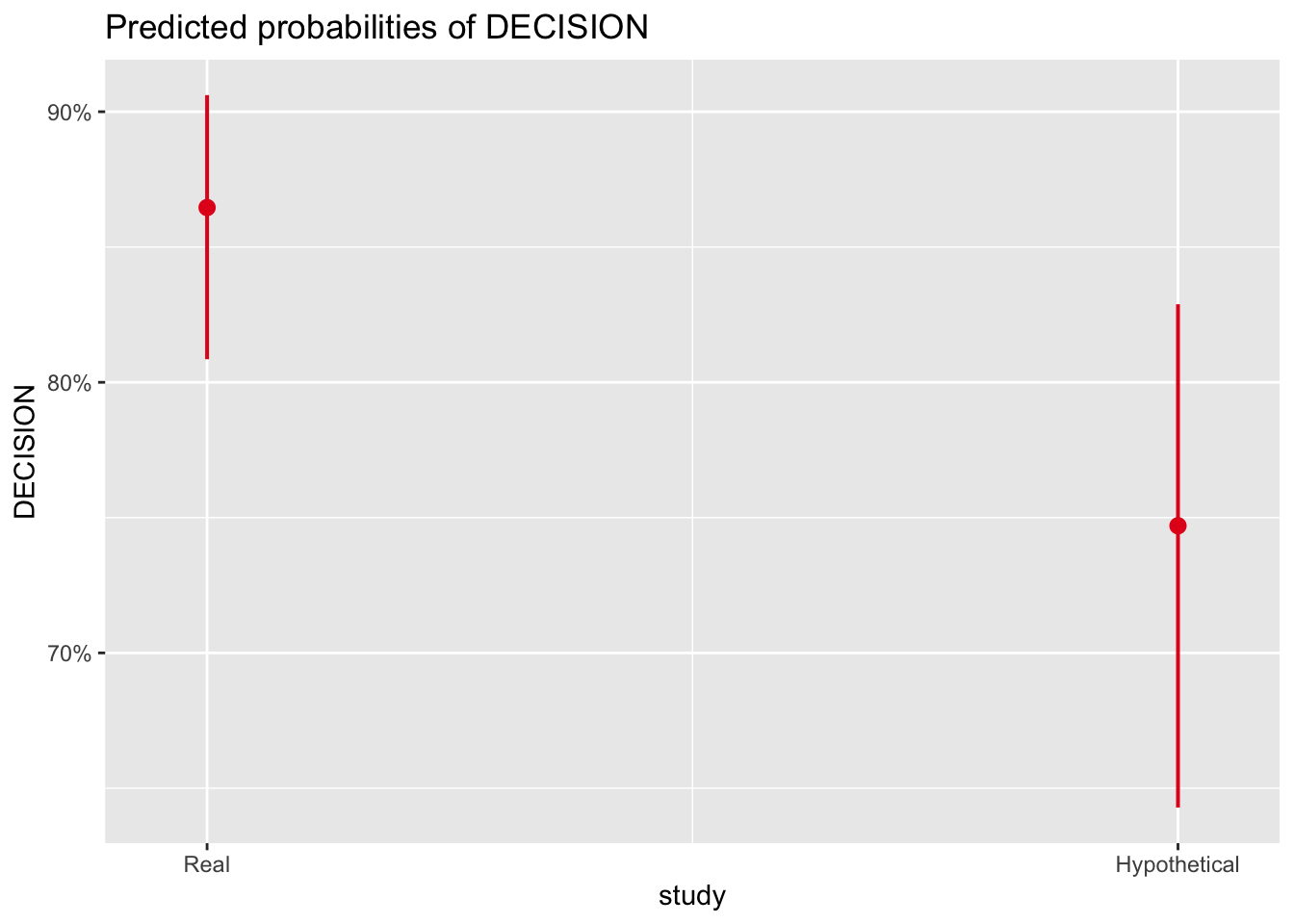
Plus some additional arguments and ggplot() layers to tidy things up. Helpfully, it recognises the y-axis is a probability and amends the scale. Unhelpfully, if you want to change the limits etc., you need to tidy the scale up again or it reverts back to proportion.

plot_model(bostyn_model2,
           type = "pred",
           terms = "study",
           axis.title = c("Real or Hypothetical Scenario", "Probability Consequentialist Decision (%)")) + 
  scale_y_continuous(labels = scales::percent, # setting to convert y to percent
                     limits = c(0.5, 1)) + # original units are proportion
  theme_classic() + 
  labs(title = "")

Scale for y is already present.
Adding another scale for y, which will replace the existing scale.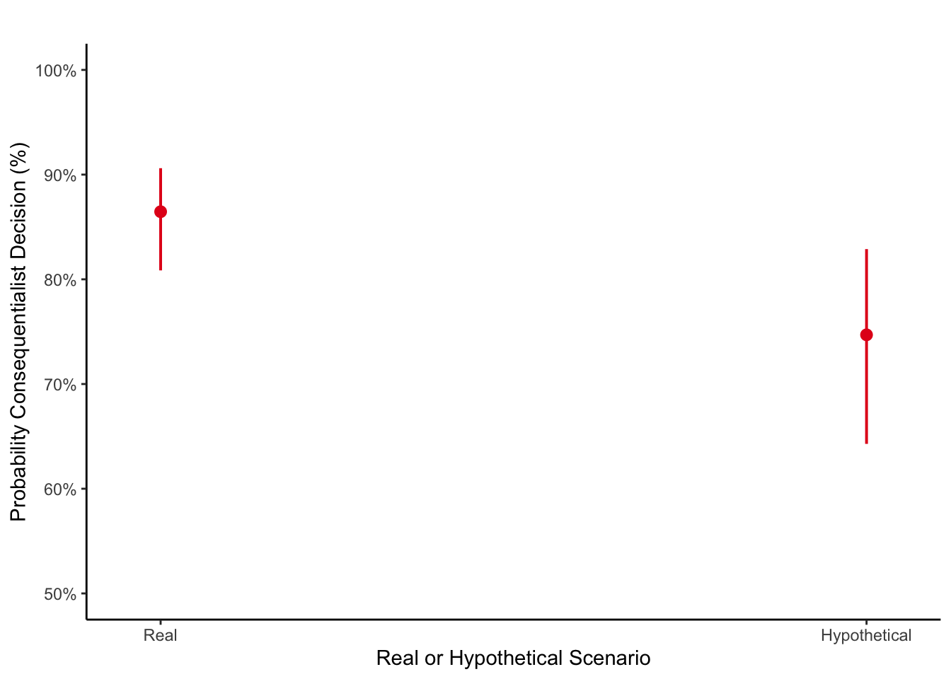

5.3 Test Yourself

Now you have followed along to a guided example, it is important you can transfer your knowledge to a new scenario. So, we have a new data set for you to try out your understanding of these techniques on. Follow the instructions below and answer the questions. The solution is there to check your answers against, but make sure you try the activities independently first.

5.3.1 Independent logistic regression

For an independent activity, we will use the same data set from Bostyn et al. (2018), but this time using a couple of extra predictors. If you are coming to this fresh, make sure to remind yourself of the data set outlined in the logistic regression section and load the data.

TipTry this

From here, apply what you learnt in the guided example for logistic regression to this new independent task and complete the questions below to check your understanding.

In Bostyn et al. (2018), they actually fit a multiple logistic regression model where they include three predictors. They include study as the key predictor of interest, but they also control for AGE and GENDER as additional predictors. Fit this model to create a new object called bostyn_model3 and answer the following questions.

• In the new model, our key predictor of study is statistically significant non-significant. The two new predictors of AGE and GENDER are statistically non-significant significant.

• The slope for study is still in log odds and negative (unless you flipped the groups). If you take the reciprocal of the exponential slope, the odds ratio for the predictor to 2 decimals is [lower 95% CI = , upper 95% CI = ].

• This suggests there are lower odds of making a consequential decision in the real hypothetical group compared to the real hypothetical group.

• Rounding to 1 decimal, the estimated probability of making a consequential decision in the real group is % (95% CI = , ) and the estimated probability in the hypothetical group is % (95% CI = , ).

CautionShow me the solution

The first step is fitting the model with three individual predictors.

bostyn_model3 <- glm(DECISION ~ study + AGE + GENDER,
                     family = binomial(link = "logit"),
                     data = bostyn_data)

summary(bostyn_model3)

Call:
glm(formula = DECISION ~ study + AGE + GENDER, family = binomial(link = "logit"), 
    data = bostyn_data)

Coefficients:
                  Estimate Std. Error z value Pr(>|z|)  
(Intercept)        -3.8900     3.4952  -1.113   0.2657  
studyHypothetical  -0.8019     0.3361  -2.385   0.0171 *
AGE                 0.3075     0.1913   1.608   0.1078  
GENDER1             0.1940     0.3920   0.495   0.6207  
---
Signif. codes:  0 '***' 0.001 '**' 0.01 '*' 0.05 '.' 0.1 ' ' 1

(Dispersion parameter for binomial family taken to be 1)

    Null deviance: 251.53  on 274  degrees of freedom
Residual deviance: 242.13  on 271  degrees of freedom
AIC: 250.13

Number of Fisher Scoring iterations: 4

Given the model, you can take the reciprocal of the exponential for the slope estimate and its 95% confidence interval. You do not need the reciprocal if you flipped the groups and estimate is above 1.

1 / exp(coef(bostyn_model3)[2])

studyHypothetical 
          2.22971 

1 / exp(confint(bostyn_model3))

Waiting for profiling to be done...

                         2.5 %     97.5 %
(Intercept)       80279.914577 0.08384154
studyHypothetical     4.312262 1.14763061
AGE                   1.040199 0.48957669
GENDER1               1.737032 0.36872266

Finally, you can calculate the estimated probability of making a consequentialist decision in each group by using the emmeans() function. If you calculated it manually with the other methods, that’s fine too.

emmeans(bostyn_model3, specs = "study")

 study        emmean    SE  df asymp.LCL asymp.UCL
 Real           1.94 0.228 Inf     1.493      2.39
 Hypothetical   1.14 0.281 Inf     0.587      1.69

Results are averaged over the levels of: GENDER 
Results are given on the logit (not the response) scale. 
Confidence level used: 0.95 

Bostyn, D. H., Sevenhant, S., & Roets, A. (2018). Of Mice, Men, and Trolleys: Hypothetical Judgment Versus Real-Life Behavior in Trolley-Style Moral Dilemmas: Psychological Science, 29(7), 1084–1093. https://doi.org/10.1177/0956797617752640

Lenth, R. V. (2024). Emmeans: Estimated marginal means, aka least-squares means. https://CRAN.R-project.org/package=emmeans

Lüdecke, D. (2024). sjPlot: Data visualization for statistics in social science. https://CRAN.R-project.org/package=sjPlot

Voas, D., & Watt, L. (2024). The odds are it’s wrong: Correcting a common mistake in statistics. Teaching Statistics. https://doi.org/10.1111/test.12391