8  Simulating Mixed Effects Models

In this chapter, we will explore linear mixed effects models by simulating data. Experimental designs that sample both subjects and stimuli from a larger population need to account for random effects of both subjects and stimuli using mixed-effects models. However, much of this research is analyzed using analysis of variance on aggregated responses because researchers are not confident specifying and interpreting mixed-effects models. This chapter will explain how to simulate data with random-effects structure (using the faux R package) and analyze the data using linear mixed-effects regression (with the lme4 R package), with a focus on interpreting the output in light of the simulated parameters. You will also learn to calculate power using simulation.

8.1 Learning objectives

By the end of this chapter, you should be able to:

1. Understand how data are structured for a linear mixed effects model

2. Be able to simulate data with a cross-classified structure

3. Understand how to run and interpret a linear mixed effects model

4. Run a power calculation for LMEM

To follow along to this chapter and try the code yourself, please download the Rmd file we will be using in this zip file.

8.2 Packages and the data sets

We will simulate data using the faux package.

library(tidyverse)   # for data wrangling, pipes, and good dataviz
library(afex)        # for mixed effect models
library(broom.mixed) # for getting tidy data tables from mixed models
library(faux)        # for simulating correlated variables

8.3 Simulation

First, we need to generate some data with the right structure for a mixed effects analysis. Here, we will simulate data for a Stroop task where subjects (sub) say the colour of colour words (stim) shown in each of two versions (congruent and incongruent). Subjects are in one of two conditions (hard or easy). The dependent variable is reaction time (`rt``).

We expect people to have faster reaction times for congruent stimuli than incongruent stimuli (main effect of version) and to be faster in the easy condition than the hard condition (main effect of condition). We’ll look at some different interaction patterns below.

8.3.1 Random Factors

First, set up the overall structure of your data by specifying the number of observations for each random factor. Here, we have a crossed design, so each subject responds to each stimulus. We’ll set the numbers to small numbers as a demo first.

sub_n  <- 2 # number of subjects in this simulation
stim_n  <- 2 # number of stimuli in this simulation

dat <- add_random(sub = sub_n) |>
  add_random(stim = stim_n)

dat

sub	stim
sub1	stim1
sub1	stim2
sub2	stim1
sub2	stim2

8.3.2 Fixed Factors

Next, add the fixed factors. Specify if they vary between one of the random factors and specify the names of the levels.

Each subject is in only one condition, so the code below assigns half easy and half hard. You can change the proportion of subjects assigned each level with the .prob argument.

Stimuli are seen in both congruent and incongruent versions, so this will double the number of rows in our resulting data set.

sub_n  <- 2 # number of subjects in this simulation
stim_n  <- 2 # number of stimuli in this simulation

dat <- add_random(sub = sub_n) |>
  add_random(stim = stim_n) |>
  add_between(.by = "sub", condition = c("easy","hard")) |>
  add_within(version = c("congruent", "incongruent"))

dat

sub	stim	condition	version
sub1	stim1	easy	congruent
sub1	stim1	easy	incongruent
sub1	stim2	easy	congruent
sub1	stim2	easy	incongruent
sub2	stim1	hard	congruent
sub2	stim1	hard	incongruent
sub2	stim2	hard	congruent
sub2	stim2	hard	incongruent

8.3.3 Contrast Coding

To be able to calculate the dependent variable, you need to recode categorical variables into numbers. Use the helper function add_contrast() for this. The code below creates anova-coded versions of condition and version. Luckily for us, the factor levels default to a sensible order, with “easy” predicted to have a faster (lower) reactive time than “hard”, and “congruent” predicted to have a faster RT than “incongruent”, but we can also customise the order of levels with add_contrast(); see the contrasts vignette for more details.

sub_n  <- 2 # number of subjects in this simulation
stim_n  <- 2 # number of stimuli in this simulation

dat <- add_random(sub = sub_n) |>
  add_random(stim = stim_n) |>
  add_between(.by = "sub", condition = c("easy","hard")) |>
  add_within(version = c("congruent", "incongruent")) |>
  add_contrast("condition") |>
  add_contrast("version")

dat

sub	stim	condition	version	condition.hard-easy	version.incongruent-congruent
sub1	stim1	easy	congruent	-0.5	-0.5
sub1	stim1	easy	incongruent	-0.5	0.5
sub1	stim2	easy	congruent	-0.5	-0.5
sub1	stim2	easy	incongruent	-0.5	0.5
sub2	stim1	hard	congruent	0.5	-0.5
sub2	stim1	hard	incongruent	0.5	0.5
sub2	stim2	hard	congruent	0.5	-0.5
sub2	stim2	hard	incongruent	0.5	0.5

The function defaults to very descriptive names that help you interpret the fixed factors. Here, “condition.hard-easy” means the main effect of this factor is interpreted as the RT for hard trials minus the RT for easy trials, and “version.incongruent-congruent” means the main effect of this factor is interpreted as the RT for incongruent trials minus the RT for congruent trials. However, we can change these to simpler labels with the colnames argument.

8.3.4 Random Effects

Now we specify the random effect structure. We’ll just add random intercepts to start, but will cover random slopes later.

Each subject will have slightly faster or slower reaction times on average; this is their random intercept (sub_i). We’ll model it from a normal distribution with a mean of 0 and SD of 100ms.

Each stimulus will have slightly faster or slower reaction times on average; this is their random intercept (stim_i). We’ll model it from a normal distribution with a mean of 0 and SD of 50ms (it seems reasonable to expect less variability between words than people for this task).

Run this code a few times to see how the random effects change each time. this is because they are sampled from populations.

sub_n  <- 2 # number of subjects in this simulation
stim_n  <- 2 # number of stimuli in this simulation
sub_sd <- 100 # SD for the subjects' random intercept
stim_sd <- 50 # SD for the stimuli's random intercept

dat <- add_random(sub = sub_n) |>
  add_random(stim = stim_n) |>
  add_between(.by = "sub", condition = c("easy","hard")) |>
  add_within(version = c("congruent", "incongruent")) |>
  add_contrast("condition", colnames = "cond") |>
  add_contrast("version", colnames = "vers") |>
  add_ranef(.by = "sub", sub_i = sub_sd) |>
  add_ranef(.by = "stim", stim_i = stim_sd)

dat

sub	stim	condition	version	cond	vers	sub_i	stim_i
sub1	stim1	easy	congruent	-0.5	-0.5	31.081574	-32.53293
sub1	stim1	easy	incongruent	-0.5	0.5	31.081574	-32.53293
sub1	stim2	easy	congruent	-0.5	-0.5	31.081574	14.08654
sub1	stim2	easy	incongruent	-0.5	0.5	31.081574	14.08654
sub2	stim1	hard	congruent	0.5	-0.5	9.159506	-32.53293
sub2	stim1	hard	incongruent	0.5	0.5	9.159506	-32.53293
sub2	stim2	hard	congruent	0.5	-0.5	9.159506	14.08654
sub2	stim2	hard	incongruent	0.5	0.5	9.159506	14.08654

8.3.5 Error Term

Finally, add an error term. This uses the same add_ranef() function, just without specifying which random factor it’s for with .by. In essence, this samples an error value from a normal distribution with a mean of 0 and the specified SD for each trial. We’ll also increase the number of subjects and stimuli to more realistic values now.

sub_n    <- 200 # number of subjects in this simulation
stim_n   <- 50  # number of stimuli in this simulation
sub_sd   <- 100 # SD for the subjects' random intercept
stim_sd  <- 50  # SD for the stimuli's random intercept
error_sd <- 25  # residual (error) SD

dat <- add_random(sub = sub_n) |>
  add_random(stim = stim_n) |>
  add_between(.by = "sub", condition = c("easy","hard")) |>
  add_within(version = c("congruent", "incongruent")) |>
  add_contrast("condition", colnames = "cond") |>
  add_contrast("version", colnames = "vers") |>
  add_ranef(.by = "sub", sub_i = sub_sd) |>
  add_ranef(.by = "stim", stim_i = stim_sd) |>
  add_ranef(err = error_sd)

8.3.6 Calculate the DV

Now we can calculate the dependent variable (rt) by adding together an overall intercept (mean reaction time for all trials), the subject-specific intercept, the stimulus-specific intercept, and an error term, plus the effect of subject condition, the effect of stimulus version, and the interaction between condition and version.

We set these effects in raw units (ms). So when we set the effect of subject condition (sub_cond_eff) to 50, that means the average difference between the easy and hard condition is 50ms. Easy was coded as -0.5 and hard was coded as +0.5, which means that trials in the easy condition have -0.5 * 50ms (i.e., -25ms) added to their reaction time, while trials in the hard condition have +0.5 * 50ms (i.e., +25ms) added to their reaction time.

sub_n         <- 200 # number of subjects in this simulation
stim_n        <- 50  # number of stimuli in this simulation
sub_sd        <- 100 # SD for the subjects' random intercept
stim_sd       <- 50  # SD for the stimuli's random intercept
error_sd      <- 25  # residual (error) SD
grand_i       <- 400 # overall mean rt
cond_eff      <- 50  # mean difference between conditions: hard - easy
vers_eff      <- 50  # mean difference between versions: incongruent - congruent
cond_vers_ixn <-  0  # interaction between version and condition

dat <- add_random(sub = sub_n) |>
  add_random(stim = stim_n) |>
  add_between(.by = "sub", condition = c("easy","hard")) |>
  add_within(version = c("congruent", "incongruent")) |>
  add_contrast("condition", colnames = "cond") |>
  add_contrast("version", colnames = "vers") |>
  add_ranef(.by = "sub", sub_i = sub_sd) |>
  add_ranef(.by = "stim", stim_i = stim_sd) |>
  add_ranef(err = error_sd) |>
  mutate(rt = grand_i + sub_i + stim_i + err +
         (cond * cond_eff) + 
         (vers * vers_eff) + 
         (cond * vers * cond_vers_ixn) # in this example, this is always 0 and could be omitted
  )

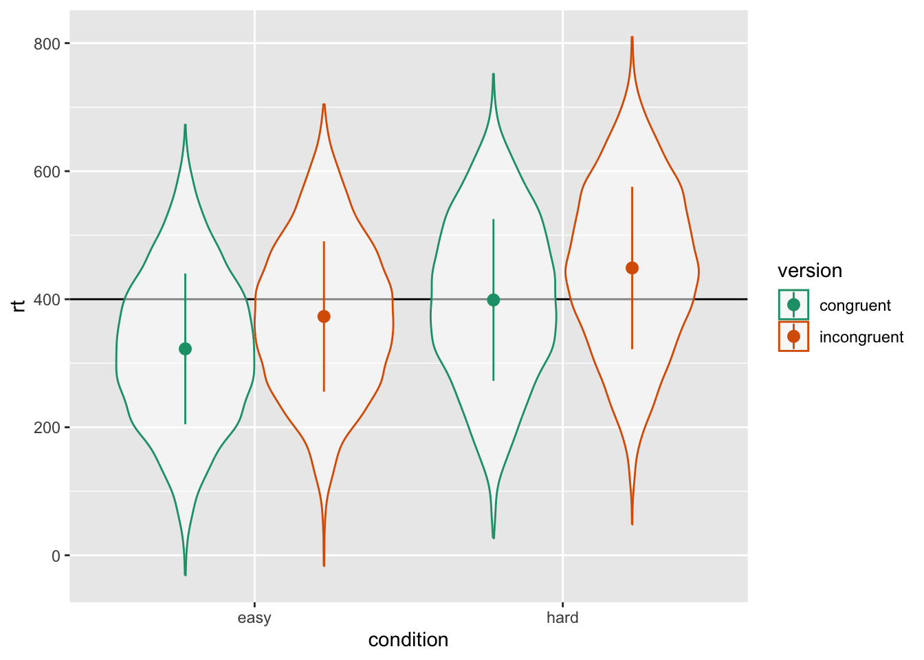
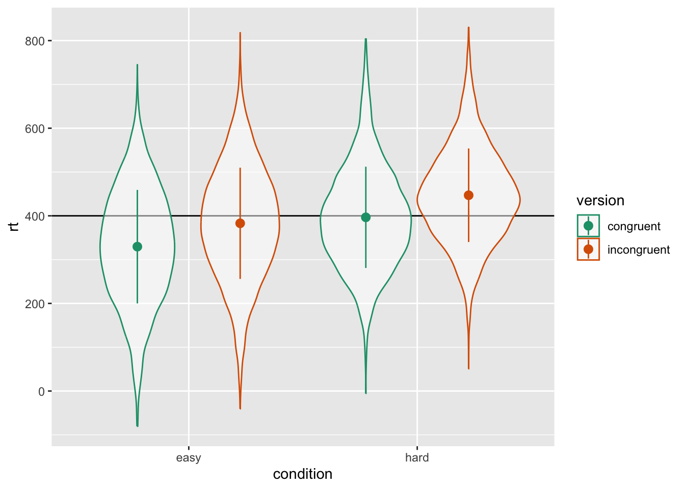
As always, graph to make sure you’ve simulated the general pattern you expected.

ggplot(dat, aes(condition, rt, color = version)) +
  geom_hline(yintercept = grand_i) +
  geom_violin(alpha = 0.5) +
  stat_summary(fun = mean,
               fun.min = \(x){mean(x) - sd(x)},
               fun.max = \(x){mean(x) + sd(x)},
               position = position_dodge(width = 0.9)) +
  scale_color_brewer(palette = "Dark2")

Double-check the simulated pattern

8.3.7 Interactions

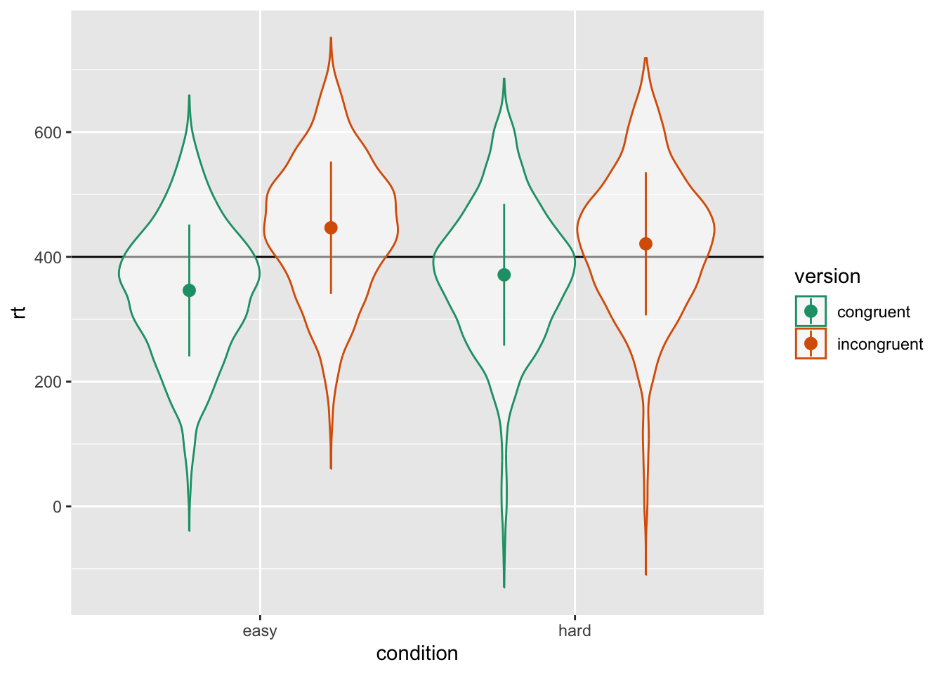
If you want to simulate an interaction, it can sometimes be tricky to figure out what to set the main effects and interaction effect to. It can often be easier to think about the simple main effects for each cell. Create four new variables and set them to the deviations from the overall mean you’d expect for each condition (so they should add up to 0). Here, we’re simulating a small effect of version in the hard condition (50ms difference) and double that effect of version in the easy condition (100ms difference).

# set variables to use in calculations below
easy_congr <- -50
easy_incon <- +50
hard_congr <- -25
hard_incon <- +25

Use the code below to transform the simple main effects above into main effects and interactions for use in the equations below. This uses the sim_design() function from faux to set up a fixed-design simulated sample with the exact cell means above (using empirical = TRUE), runs a linear model on the data, and extracts the coefficients. This only works if you contrast-code the factors in the same way, and use the same formula as your LMEM. It doesn’t matter if you set the factors to between or within for this, so it’s easiest to set them all to between.

# simulated the data
fixed_data <- sim_design(
  between = list(condition = c("easy","hard"),
                 version   = c("congruent", "incongruent")),
  mu = c(easy_congr, easy_incon, hard_congr, hard_incon),
  dv = "rt",
  empirical = TRUE,
  plot = FALSE
) |>
  # add the same contrasts you'll use in your LMEM 
  add_contrast("condition", colnames = "cond") |>
  add_contrast("version", colnames = "vers")

# run the same formula using lm()
fixed_model <- lm(rt ~ cond * vers, data = fixed_data)

# extract and round the coefficients
fixed_coefs <- coef(fixed_model) |> round(2)

# assign the coefficients to the relevant variables
cond_eff <- fixed_coefs["cond"]
vers_eff <- fixed_coefs["vers"]
cond_vers_ixn <- fixed_coefs["cond:vers"]

Then generate the rt the same way we did above, but also add the interaction effect multiplied by the effect-coded subject condition and stimulus version.

dat <- add_random(sub = sub_n) |>
  add_random(stim = stim_n) |>
  add_between(.by = "sub", condition = c("easy","hard")) |>
  add_within(version = c("congruent", "incongruent")) |>
  add_contrast("condition", colnames = "cond") |>
  add_contrast("version", colnames = "vers") |>
  add_ranef(.by = "sub", sub_i = sub_sd) |>
  add_ranef(.by = "stim", stim_i = stim_sd) |>
  add_ranef(err = error_sd) |>
  mutate(rt = grand_i + sub_i + stim_i + err +
         (cond * cond_eff) + 
         (vers * vers_eff) + 
         (cond * vers * cond_vers_ixn)
  )

ggplot(dat, aes(condition, rt, color = version)) +
  geom_hline(yintercept = grand_i) +
  geom_violin(alpha = 0.5) +
  stat_summary(fun = mean,
               fun.min = \(x){mean(x) - sd(x)},
               fun.max = \(x){mean(x) + sd(x)},
               position = position_dodge(width = 0.9)) +
  scale_color_brewer(palette = "Dark2")

Double-check the interaction between condition and version

group_by(dat, condition, version) %>%
  summarise(m = mean(rt) - grand_i %>% round(1),
            .groups = "drop") %>%
  pivot_wider(names_from = version, 
              values_from = m)

condition	congruent	incongruent
easy	-53.81441	46.64935
hard	-28.78197	20.91479

8.4 Analysis

Now we will run a linear mixed effects model with lmer and look at the summary.

mod <- lmer(rt ~ cond * vers +
              (1 | sub) + 
              (1 | stim),
            data = dat)

mod.sum <- summary(mod)

mod.sum

Linear mixed model fit by REML. t-tests use Satterthwaite's method [
lmerModLmerTest]
Formula: rt ~ cond * vers + (1 | sub) + (1 | stim)
   Data: dat

REML criterion at convergence: 187241.2

Scaled residuals: 
    Min      1Q  Median      3Q     Max 
-3.9082 -0.6736  0.0081  0.6720  3.8481 

Random effects:
 Groups   Name        Variance Std.Dev.
 sub      (Intercept) 10119.8  100.60  
 stim     (Intercept)  1521.5   39.01  
 Residual               622.8   24.96  
Number of obs: 20000, groups:  sub, 200; stim, 50

Fixed effects:
              Estimate Std. Error         df t value Pr(>|t|)    
(Intercept)   396.2419     9.0033   206.0932  44.011   <2e-16 ***
cond           -0.3511    14.2310   198.0056  -0.025     0.98    
vers           75.0803     0.3529 19748.9984 212.730   <2e-16 ***
cond:vers     -50.7670     0.7059 19748.9984 -71.921   <2e-16 ***
---
Signif. codes:  0 '***' 0.001 '**' 0.01 '*' 0.05 '.' 0.1 ' ' 1

Correlation of Fixed Effects:
          (Intr) cond  vers 
cond      0.000             
vers      0.000  0.000      
cond:vers 0.000  0.000 0.000

8.4.1 Sense checks

First, check that your groups make sense.

• The number of obs should be the total number of trials analysed.
• sub should be what we set sub_n to above.
• stim should be what we set stim_n to above.

Random.Fator	value	parameters
sub	200	200
stim	50	50

Next, look at the random effects.

• The SD for sub should be near sub_sd.
• The SD for stim should be near stim_sd.
• The residual SD should be near error_sd.

Groups	Name	SD	parameters
sub	(Intercept)	101	100
stim	(Intercept)	39	50
Residual	NA	25	25

Finally, look at the fixed effects.

• The estimate for the Intercept should be near the grand_i.
• The main effect of cond should be near what we calculated for cond_eff.
• The main effect of vers should be near what we calculated for vers_eff.
• The interaction between cond:vers should be near what we calculated for cond_vers_ixn.

Effect	Estimate	parameters
(Intercept)	396	400
cond	0	0
vers	75	75
cond:vers	-51	-50

8.4.2 Random effects

Plot the subject intercepts from our code above (dat$sub_i) against the subject intercepts calculated by lmer (ranef(mod)$sub_id).

# get simulated random intercept for each subject
sub_sim <- dat |>
  group_by(sub, sub_i) |>
  summarise(.groups = "drop")

# join to calculated random intercept from model
sub_sim_mod <- ranef(mod)$sub |>
  as_tibble(rownames = "sub") |>
  rename(mod_sub_i = `(Intercept)`) |>
  left_join(sub_sim, by = "sub")

# plot to check correspondence
sub_sim_mod |>
  ggplot(aes(sub_i,mod_sub_i)) +
  geom_point() +
  geom_smooth(method = "lm", formula = y~x) +
  xlab("Simulated random intercepts (sub_i)") +
  ylab("Modeled random intercepts")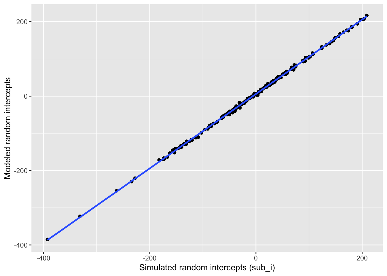

Compare simulated subject random intercepts to those from the model

Plot the stimulus intercepts from our code above (dat$stim_i) against the stimulus intercepts calculated by lmer (ranef(mod)$stim_id).

# get simulated random intercept for each stimulus
stim_sim <- dat |>
  group_by(stim, stim_i) |>
  summarise(.groups = "drop")

# join to calculated random intercept from model
stim_sim_mod <- ranef(mod)$stim |>
  as_tibble(rownames = "stim") |>
  rename(mod_stim_i = `(Intercept)`) |>
  left_join(stim_sim, by = "stim")

# plot to check correspondence
stim_sim_mod |>
  ggplot(aes(stim_i,mod_stim_i)) +
  geom_point() +
  geom_smooth(method = "lm", formula = y~x) +
  xlab("Simulated random intercepts (stim_i)") +
  ylab("Modeled random intercepts")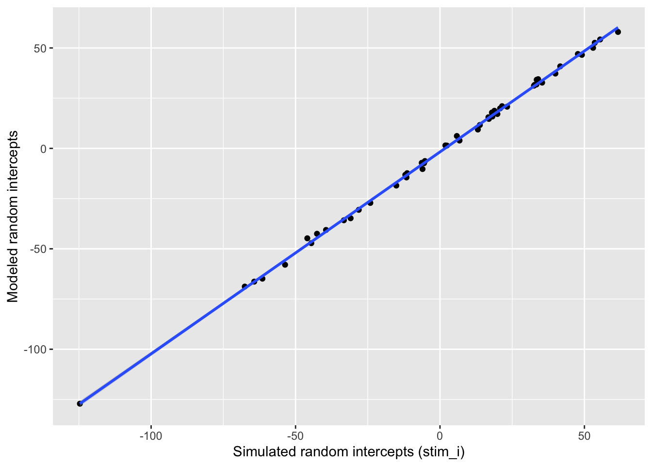

Compare simulated stimulus random intercepts to those from the model

8.4.3 Function

You can put the code above in a function so you can run it more easily and change the parameters. I removed the plot and set the argument defaults to the same as the example above with all fixed effects set to 0, but you can set them to other patterns.

sim_lmer <- function( sub_n = 200,
                      stim_n = 50,
                      sub_sd = 100,
                      stim_sd = 50,
                      error_sd = 25,
                      grand_i = 400,
                      cond_eff = 0,
                      vers_eff = 0, 
                      cond_vers_ixn = 0) {
  dat <- add_random(sub = sub_n) |>
    add_random(stim = stim_n) |>
    add_between(.by = "sub", condition = c("easy","hard")) |>
    add_within(version = c("congruent", "incongruent")) |>
    add_contrast("condition", colnames = "cond") |>
    add_contrast("version", colnames = "vers") |>
    add_ranef(.by = "sub", sub_i = sub_sd) |>
    add_ranef(.by = "stim", stim_i = stim_sd) |>
    add_ranef(err = error_sd) |>
    mutate(rt = grand_i + sub_i + stim_i + err +
           (cond * cond_eff) + 
           (vers * vers_eff) + 
           (cond * vers * cond_vers_ixn)
    )
  
  mod <- lmer(rt ~ cond * vers +
                (1 | sub) + 
                (1 | stim),
              data = dat)
  
  return(mod)
}

Run the function with the default values (so all fixed effects set to 0).

sim_lmer() %>% summary()

Linear mixed model fit by REML. t-tests use Satterthwaite's method [
lmerModLmerTest]
Formula: rt ~ cond * vers + (1 | sub) + (1 | stim)
   Data: dat

REML criterion at convergence: 187250.8

Scaled residuals: 
    Min      1Q  Median      3Q     Max 
-4.0463 -0.6723 -0.0033  0.6689  4.0546 

Random effects:
 Groups   Name        Variance Std.Dev.
 sub      (Intercept) 9867.6   99.34   
 stim     (Intercept) 2462.7   49.63   
 Residual              622.5   24.95   
Number of obs: 20000, groups:  sub, 200; stim, 50

Fixed effects:
              Estimate Std. Error         df t value Pr(>|t|)    
(Intercept)  3.903e+02  9.931e+00  1.572e+02  39.299   <2e-16 ***
cond        -3.609e+01  1.405e+01  1.980e+02  -2.568    0.011 *  
vers         4.512e-03  3.529e-01  1.975e+04   0.013    0.990    
cond:vers    1.072e+00  7.057e-01  1.975e+04   1.519    0.129    
---
Signif. codes:  0 '***' 0.001 '**' 0.01 '*' 0.05 '.' 0.1 ' ' 1

Correlation of Fixed Effects:
          (Intr) cond  vers 
cond      0.000             
vers      0.000  0.000      
cond:vers 0.000  0.000 0.000

Try changing some variables to simulate different patterns of fixed effects.

sim_lmer(cond_eff = 0,
         vers_eff = 75, 
         cond_vers_ixn = -50) %>%
  summary()

Linear mixed model fit by REML. t-tests use Satterthwaite's method [
lmerModLmerTest]
Formula: rt ~ cond * vers + (1 | sub) + (1 | stim)
   Data: dat

REML criterion at convergence: 187336.1

Scaled residuals: 
    Min      1Q  Median      3Q     Max 
-3.7202 -0.6692  0.0031  0.6675  4.6586 

Random effects:
 Groups   Name        Variance Std.Dev.
 sub      (Intercept) 10790.0  103.87  
 stim     (Intercept)  2153.8   46.41  
 Residual               624.9   25.00  
Number of obs: 20000, groups:  sub, 200; stim, 50

Fixed effects:
              Estimate Std. Error         df t value Pr(>|t|)    
(Intercept)   400.8716     9.8518   178.9542  40.690   <2e-16 ***
cond           -1.7296    14.6944   197.9927  -0.118    0.906    
vers           75.2895     0.3535 19749.0020 212.971   <2e-16 ***
cond:vers     -49.2259     0.7070 19749.0020 -69.623   <2e-16 ***
---
Signif. codes:  0 '***' 0.001 '**' 0.01 '*' 0.05 '.' 0.1 ' ' 1

Correlation of Fixed Effects:
          (Intr) cond  vers 
cond      0.000             
vers      0.000  0.000      
cond:vers 0.000  0.000 0.000

TipTry this

How would you modify the function above to take the input of the four cell means (easy_congr, easy_incon hard_congr, hard_incon), instead of the coefficients (cond_eff, vers_eff, cond_vers_ixn)?

8.4.4 Power analysis

Calculating power for a LMEM can seem really tricky, but if you can simulate the data you expect, you can calculate power for anything!

First, wrap your simulation function inside of another function that takes the argument of a replication number, runs a simulated analysis, and returns a data table of the fixed and random effects (made with broom.mixed::tidy()). You can use purrr’s map_df() function to create a data table of results from multiple replications of this function. We’re only running 10 replications here in the interests of time, but you’ll want to run 100 or more for a proper power calculation.

sim_lmer_pwr <- function(rep) {
  s <- sim_lmer(cond_eff = 0,
                vers_eff = 75, 
                cond_vers_ixn = 50)
  
  # put just the fixed effects into a data table
  broom.mixed::tidy(s, "fixed") %>%
    mutate(rep = rep) # add a column for which rep
}

my_power <- map_df(1:10, sim_lmer_pwr)

You can then plot the distribution of estimates across your simulations.

ggplot(my_power, aes(estimate, color = term)) +
  geom_density() +
  facet_wrap(~term, scales = "free")

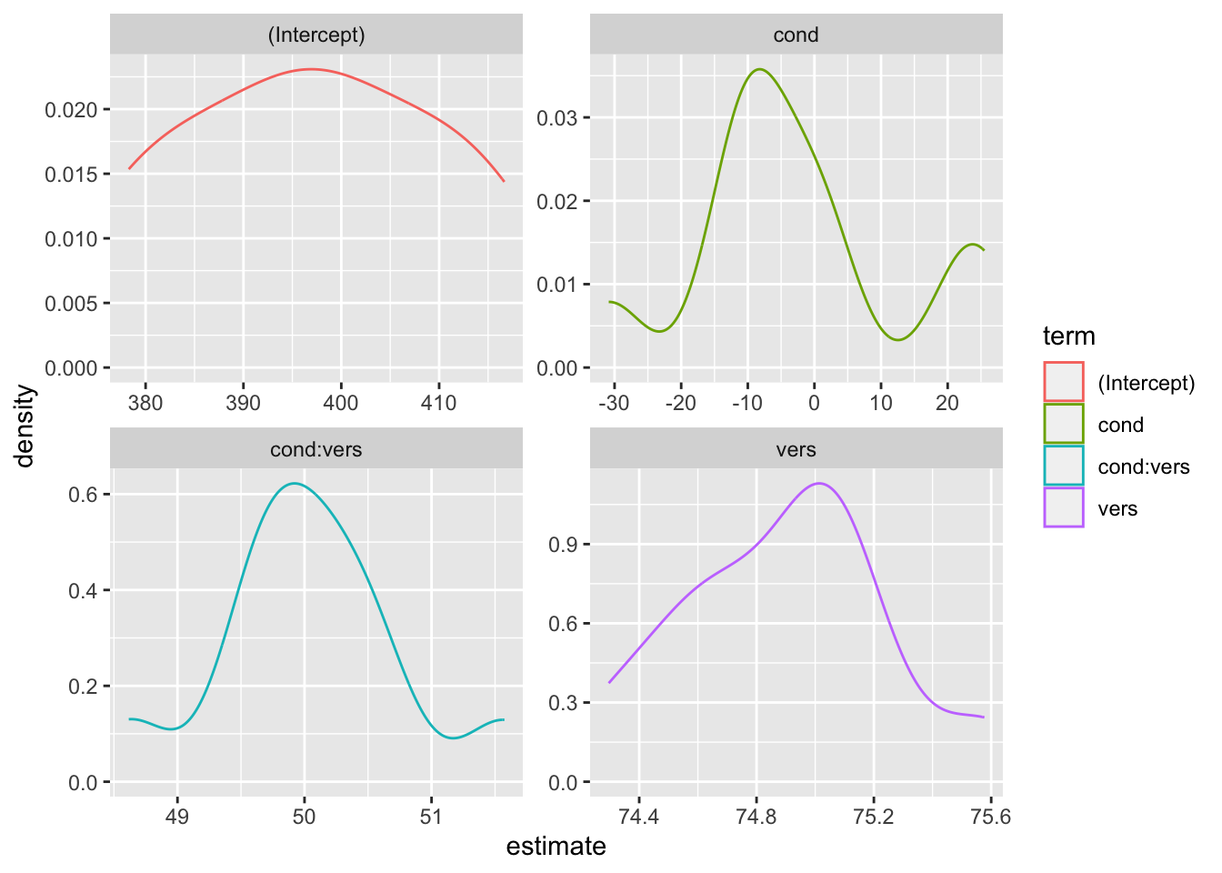
You can also just calculate power as the proportion of p-values less than your alpha.

my_power %>%
  group_by(term) %>%
  summarise(power = mean(p.value < 0.05),
            .groups = "drop")

term	power
(Intercept)	1.0
cond	0.1
cond:vers	1.0
vers	1.0

8.5 Random slopes

In the example so far we’ve ignored random variation among subjects or stimuli in the size of the fixed effects (i.e., random slopes).

First, let’s reset the parameters we set above.

sub_n         <- 200 # number of subjects in this simulation
stim_n        <- 50  # number of stimuli in this simulation
sub_sd        <- 100 # SD for the subjects' random intercept
stim_sd       <- 50  # SD for the stimuli's random intercept
error_sd      <- 25  # residual (error) SD
grand_i       <- 400 # overall mean rt
cond_eff      <- 50  # mean difference between conditions: hard - easy
vers_eff      <- 50  # mean difference between versions: incongruent - congruent
cond_vers_ixn <-  0  # interaction between version and condition

8.5.1 Slopes

In addition to generating a random intercept for each subject, now we will also generate a random slope for any within-subject factors. The only within-subject factor in this design is version. The main effect of version is set to 50 above, but different subjects will show variation in the size of this effect. That’s what the random slope captures. We’ll set sub_vers_sd below to the SD of this variation and use this to calculate the random slope (sub_version_slope) for each subject.

Also, it’s likely that the variation between subjects in the size of the effect of version is related in some way to between-subject variation in the intercept. So we want the random intercept and slope to be correlated. Here, we’ll simulate a case where subjects who have slower (larger) reaction times across the board show a smaller effect of condition, so we set sub_i_vers_cor below to a negative number (-0.2).

We just have to edit the first add_ranef() to add two variables (sub_i, sub_vers_slope) that are correlated with r = -0.2, means of 0, and SDs equal to what we set sub_sd above and sub_vers_sd below.

sub_vers_sd <- 20
sub_i_vers_cor <- -0.2

dat <- add_random(sub = sub_n) |>
    add_random(stim = stim_n) |>
    add_between(.by = "sub", condition = c("easy","hard")) |>
    add_within(version = c("congruent", "incongruent")) |>
    add_contrast("condition", colnames = "cond") |>
    add_contrast("version", colnames = "vers") |>
    add_ranef(.by = "sub", sub_i = sub_sd, 
              sub_vers_slope = sub_vers_sd,
              .cors = sub_i_vers_cor)

8.5.2 Correlated Slopes

In addition to generating a random intercept for each stimulus, we will also generate a random slope for any within-stimulus factors. Both version and condition are within-stimulus factors (i.e., all stimuli are seen in both congruent and incongruent versions and both easy and hard conditions). So the main effects of version and condition (and their interaction) will vary depending on the stimulus.

They will also be correlated, but in a more complex way than above. You need to set the correlations for all pairs of slopes and intercept. Let’s set the correlation between the random intercept and each of the slopes to -0.4 and the slopes all correlate with each other +0.2 (You could set each of the six correlations separately if you want, though).

stim_vers_sd <- 10 # SD for the stimuli's random slope for stim_version
stim_cond_sd <- 30 # SD for the stimuli's random slope for sub_cond
stim_cond_vers_sd <- 15 # SD for the stimuli's random slope for sub_cond:stim_version
stim_i_cor <- -0.4 # correlations between intercept and slopes
stim_s_cor <- +0.2 # correlations among slopes

# specify correlations for rnorm_multi (one of several methods)
stim_cors <- c(stim_i_cor, stim_i_cor, stim_i_cor,
                           stim_s_cor, stim_s_cor,
                                       stim_s_cor)

dat <- add_random(sub = sub_n) |>
    add_random(stim = stim_n) |>
    add_between(.by = "sub", condition = c("easy","hard")) |>
    add_within(version = c("congruent", "incongruent")) |>
    add_contrast("condition", colnames = "cond") |>
    add_contrast("version", colnames = "vers") |>
    add_ranef(.by = "sub", sub_i = sub_sd, 
              sub_vers_slope = sub_vers_sd,
              .cors = sub_i_vers_cor) |>
    add_ranef(.by = "stim", stim_i = stim_sd,
              stim_vers_slope = stim_vers_sd,
              stim_cond_slope = stim_cond_sd,
              stim_cond_vers_slope = stim_cond_vers_sd,
              .cors = stim_cors)

8.5.3 Calculate the DV

Now we can calculate the rt by adding together an overall intercept (mean RT for all trials), the subject-specific intercept, the stimulus-specific intercept, the effect of subject condition, the stimulus-specific slope for condition, the effect of stimulus version, the stimulus-specific slope for version, the subject-specific slope for condition, the interaction between condition and version (set to 0 for this example), the stimulus-specific slope for the interaction between condition and version, and an error term.

dat <- add_random(sub = sub_n) |>
    add_random(stim = stim_n) |>
    add_between(.by = "sub", condition = c("easy","hard")) |>
    add_within(version = c("congruent", "incongruent")) |>
    add_contrast("condition", colnames = "cond") |>
    add_contrast("version", colnames = "vers") |>
    add_ranef(.by = "sub", sub_i = sub_sd, 
              sub_vers_slope = sub_vers_sd,
              .cors = sub_i_vers_cor) |>
    add_ranef(.by = "stim", stim_i = stim_sd,
              stim_vers_slope = stim_vers_sd,
              stim_cond_slope = stim_cond_sd,
              stim_cond_vers_slope = stim_cond_vers_sd,
              .cors = stim_cors) |>
    add_ranef(err = error_sd) |>
  mutate(
    trial_cond_eff = cond_eff + stim_cond_slope,
    trial_vers_eff = vers_eff + sub_vers_slope + stim_vers_slope,
    trial_cond_vers_ixn = cond_vers_ixn + stim_cond_vers_slope,
    rt = grand_i + sub_i + stim_i + err +
         (cond * trial_cond_eff) + 
         (vers * trial_vers_eff) + 
         (cond * vers * trial_cond_vers_ixn)
  )

As always, graph to make sure you’ve simulated the general pattern you expected.

ggplot(dat, aes(condition, rt, color = version)) +
  geom_hline(yintercept = grand_i) +
  geom_violin(alpha = 0.5) +
  stat_summary(fun = mean,
               fun.min = \(x){mean(x) - sd(x)},
               fun.max = \(x){mean(x) + sd(x)},
               position = position_dodge(width = 0.9)) +
  scale_color_brewer(palette = "Dark2")

Double-check the simulated pattern

8.6 Analysis

New we’ll run a linear mixed effects model with lmer and look at the summary. You specify random slopes by adding the within-level effects to the random intercept specifications. Since the only within-subject factor is version, the random effects specification for subjects is (1 + vers | sub). Since both condition and version are within-stimuli factors, the random effects specification for stimuli is (1 + vers*cond | stim).

This model will take a lot longer to run than one without random slopes specified. This might be a good time for a coffee break.

mod <- lmer(rt ~ cond * vers +
              (1 + vers | sub) + 
              (1 + vers*cond | stim),
            data = dat)

Warning in checkConv(attr(opt, "derivs"), opt$par, ctrl = control$checkConv, :
Model failed to converge with max|grad| = 0.00288246 (tol = 0.002, component 1)

mod.sum <- summary(mod)

mod.sum

Linear mixed model fit by REML. t-tests use Satterthwaite's method [
lmerModLmerTest]
Formula: rt ~ cond * vers + (1 + vers | sub) + (1 + vers * cond | stim)
   Data: dat

REML criterion at convergence: 188501.1

Scaled residuals: 
    Min      1Q  Median      3Q     Max 
-4.3519 -0.6690 -0.0015  0.6606  3.7820 

Random effects:
 Groups   Name        Variance Std.Dev. Corr             
 sub      (Intercept) 10022.56 100.113                   
          vers          465.19  21.568  -0.19            
 stim     (Intercept)  3553.02  59.607                   
          vers           97.96   9.897  -0.51            
          cond          903.82  30.064  -0.52  0.53      
          vers:cond     315.50  17.762  -0.47  0.33  0.40
 Residual               628.47  25.069                   
Number of obs: 20000, groups:  sub, 200; stim, 50

Fixed effects:
            Estimate Std. Error      df t value Pr(>|t|)    
(Intercept)  389.016     11.009 126.838  35.335  < 2e-16 ***
cond          65.491     14.787 227.692   4.429 1.47e-05 ***
vers          51.857      2.100 163.402  24.692  < 2e-16 ***
cond:vers     -2.879      4.015 181.259  -0.717    0.474    
---
Signif. codes:  0 '***' 0.001 '**' 0.01 '*' 0.05 '.' 0.1 ' ' 1

Correlation of Fixed Effects:
          (Intr) cond   vers  
cond      -0.113              
vers      -0.348  0.102       
cond:vers -0.225 -0.067  0.139
optimizer (nloptwrap) convergence code: 0 (OK)
Model failed to converge with max|grad| = 0.00288246 (tol = 0.002, component 1)

8.6.1 Sense checks

First, check that your groups make sense.

• sub = sub_n (200)
• stim = stim_n (50)

Random.Fator	value	parameters
sub	200	200
stim	50	50

Next, look at the SDs for the random effects.

• Group:sub
  • (Intercept) ~= sub_sd
  • vers ~= sub_vers_sd
• Group: stim
  • (Intercept) ~= stim_sd
  • vers ~= stim_vers_sd
  • cond ~= stim_cond_sd
  • vers:cond ~= stim_cond_vers_sd
• Residual ~= error_sd

Groups	Name	SD	parameters
sub	(Intercept)	100	100
sub	vers	22	20
stim	(Intercept)	60	50
stim	vers	10	10
stim	cond	30	30
stim	vers:cond	18	15
Residual	NA	25	25

The correlations are a bit more difficult to parse. The first column under Corr shows the correlation between the random slope for that row and the random intercept. So for vers under sub, the correlation should be close to sub_i_vers_cor. For all three random slopes under stim, the correlation with the random intercept should be near stim_i_cor and their correlations with each other should be near stim_s_cor.

Finally, look at the fixed effects.

• (Intercept) ~= grand_i
• sub_cond.e ~= sub_cond_eff
• stim_version.e ~= stim_vers_eff
• sub_cond.e:stim_version.e ~= cond_vers_ixn

Effect	Estimate	parameters
(Intercept)	389	400
cond	65	50
vers	52	50
cond:vers	-3	0

8.6.2 Function

You can put the code above in a function so you can run it more easily and change the parameters. I removed the plot and set the argument defaults to the same as the example above, but you can set them to other patterns.

sim_lmer_slope <- function( sub_n = 200,
                            stim_n = 50,
                            sub_sd = 100,
                            sub_vers_sd = 20, 
                            sub_i_vers_cor = -0.2,
                            stim_sd = 50,
                            stim_vers_sd = 10,
                            stim_cond_sd = 30,
                            stim_cond_vers_sd = 15,
                            stim_i_cor = -0.4,
                            stim_s_cor = +0.2,
                            error_sd = 25,
                            grand_i = 400,
                            sub_cond_eff = 0,
                            stim_vers_eff = 0, 
                            cond_vers_ixn = 0) {
  dat <- add_random(sub = sub_n) |>
    add_random(stim = stim_n) |>
    add_between(.by = "sub", condition = c("easy","hard")) |>
    add_within(version = c("congruent", "incongruent")) |>
    add_contrast("condition", colnames = "cond") |>
    add_contrast("version", colnames = "vers") |>
    add_ranef(.by = "sub", sub_i = sub_sd, 
              sub_vers_slope = sub_vers_sd,
              .cors = sub_i_vers_cor) |>
    add_ranef(.by = "stim", stim_i = stim_sd,
              stim_vers_slope = stim_vers_sd,
              stim_cond_slope = stim_cond_sd,
              stim_cond_vers_slope = stim_cond_vers_sd,
              .cors = stim_cors) |>
    add_ranef(err = error_sd) |>
    mutate(
      trial_cond_eff = cond_eff + stim_cond_slope,
      trial_vers_eff = vers_eff + sub_vers_slope + stim_vers_slope,
      trial_cond_vers_ixn = cond_vers_ixn + stim_cond_vers_slope,
      rt = grand_i + sub_i + stim_i + err +
           (cond * trial_cond_eff) + 
           (vers * trial_vers_eff) + 
           (cond * vers * trial_cond_vers_ixn)
    )
  
  mod <- lmer(rt ~ cond * vers +
                (1 + vers | sub) + 
                (1 + vers*cond | stim),
              data = dat)
  
  return(mod)
}

Run the function with the default values (null fixed effects).

sim_lmer_slope() %>% summary()

Linear mixed model fit by REML. t-tests use Satterthwaite's method [
lmerModLmerTest]
Formula: rt ~ cond * vers + (1 + vers | sub) + (1 + vers * cond | stim)
   Data: dat

REML criterion at convergence: 188246

Scaled residuals: 
    Min      1Q  Median      3Q     Max 
-3.4659 -0.6749  0.0032  0.6728  3.6359 

Random effects:
 Groups   Name        Variance Std.Dev. Corr             
 sub      (Intercept) 9711.6   98.55                     
          vers         406.5   20.16    -0.30            
 stim     (Intercept) 2611.2   51.10                     
          vers         114.2   10.69    -0.32            
          cond        1172.0   34.24    -0.45  0.17      
          vers:cond    278.1   16.68    -0.51  0.11  0.10
 Residual              621.1   24.92                     
Number of obs: 20000, groups:  sub, 200; stim, 50

Fixed effects:
            Estimate Std. Error      df t value Pr(>|t|)    
(Intercept)  405.522     10.041 150.194  40.388  < 2e-16 ***
cond          49.549     14.758 234.689   3.357 0.000918 ***
vers          46.505      2.108 139.011  22.066  < 2e-16 ***
cond:vers     -2.403      3.767 178.933  -0.638 0.524415    
---
Signif. codes:  0 '***' 0.001 '**' 0.01 '*' 0.05 '.' 0.1 ' ' 1

Correlation of Fixed Effects:
          (Intr) cond   vers  
cond      -0.106              
vers      -0.308  0.040       
cond:vers -0.230 -0.197  0.050

Try changing some variables to simulate fixed effects.

sim_lmer_slope(sub_cond_eff = 50,
               stim_vers_eff = 50, 
               cond_vers_ixn = 0)

Warning in checkConv(attr(opt, "derivs"), opt$par, ctrl = control$checkConv, :
Model failed to converge with max|grad| = 0.00315315 (tol = 0.002, component 1)

Linear mixed model fit by REML ['lmerModLmerTest']
Formula: rt ~ cond * vers + (1 + vers | sub) + (1 + vers * cond | stim)
   Data: dat
REML criterion at convergence: 188257.2
Random effects:
 Groups   Name        Std.Dev. Corr             
 sub      (Intercept) 95.349                    
          vers        20.040   -0.19            
 stim     (Intercept) 48.210                    
          vers         8.643   -0.41            
          cond        28.119   -0.49  0.36      
          vers:cond   14.531   -0.55  0.15  0.25
 Residual             24.974                    
Number of obs: 20000, groups:  sub, 200; stim, 50
Fixed Effects:
(Intercept)         cond         vers    cond:vers  
    392.693       60.866       50.242       -0.633  
optimizer (nloptwrap) convergence code: 0 (OK) ; 0 optimizer warnings; 1 lme4 warnings 

8.7 Exercises

1. Calculate power for the parameters in the last example using the sim_lmer_slope() function.

2. Simulate data for the following design:

• 100 raters rate 50 faces from group A and 50 faces from group B
• The rt has a mean value of 50
• Group B values are 5 points higher than group A
• Rater intercepts have an SD of 5
• Face intercepts have an SD of 10
• The residual error has an SD of 8

3. For the design from exercise 2, write a function that simulates data and runs a mixed effects analysis on it.

4. The package faux has a built-in dataset called fr4. Type ?faux::fr4 into the console to view the help for this dataset. Run a mixed effects model on this dataset looking at the effect of face_sex on ratings. Remember to include a random slope for the effect of face sex and explicitly add a contrast code.

5. Use the parameters from this analysis to simulate a new dataset with 50 male and 50 female faces, and 100 raters.