Appendix E — Advanced: Dates and Times
Working with dates and times can be a little tricky, but the package in tidyverse is there to help. Their website has a helpful [cheatsheet](https://rstudio.github.io/cheatsheets/html/lubridate.html) and you can view a tutorial by typingvignette(“lubridate”)` in the console pane. The Dates and Times in R for Data Science also gives a helpful overview.
This appendix is a quick intro to some of the most useful functions for making reproducible reports.
E.1 Formats
While there is only one correct way to write date (The ISO 8601 format of “YYYY-MM-DD”), dates can be found in many formats. When you are reading a data file, you might need to specify the date format so it can be read properly. Date format specification uses abbreviations to represent the different ways people can write. the year, month, and day (as well as hours, minutes, and seconds). For example, the date 2023-01-03 is represented by the formatting string "%Y-%m-%d. The fastest way to find the list of formatting abbreviations is to look in the help for the function col_date().
Rows: 1 Columns: 4
── Column specification ────────────────────────────────────────────────────────
Delimiter: ","
chr  (3): ok, bad, terrible
date (1): best

ℹ Use `spec()` to retrieve the full column specification for this data.
ℹ Specify the column types or set `show_col_types = FALSE` to quiet this message.
You can see that only the first column read as a date, and the rest read as characters. You can set the date format using the col_types argument and two helper functions, cols() and col_date().
E.2 Parsing
The ymd functions can deal with almost all date formats, regardless of the punctuation used in the format. All of the examples below produce a date in the standard format “2022-01-03”.
See if you can make a date format that one of the parsers can’t handle.
There are similar functions for date/times, too.
[1] "2022-01-03 18:05:20 UTC"
[1] "2022-01-03 18:00:00 UTC"
The date/time functions can also take a timezone argument. If you don’t specify it, it defaults to “UTC”.
E.3 Get Parts
You frequently need to extract parts of a date/time for plotting. The following functions extract specific parts of a date or datetime object. This is a godsend for those of us who never have a clue what week of the year it is today.
# get the date and time when this function is run
now <- now(tzone = "GMT")

# get separate parts
time_parts <- list(
  second  = second(now),
  minute  = minute(now),
  hour    = hour(now),
  day     = day(now),  # day of the month (same as mday())
  wday    = wday(now), # day of the week
  yday    = yday(now), # day of the year
  week    = week(now),
  isoweek = isoweek(now), # ISO 8501 week calendar (Monday start)
  epiweek = epiweek(now), # CDC epidemiological week (Sunday Start)
  month   = month(now),
  year    = year(now),
  tz      = tz(now)
)

str(time_parts)
List of 12
$ second : num 1.27
$ minute : int 50
$ hour : int 13
$ day : int 7
$ wday : num 4
$ yday : num 7
$ week : num 1
$ isoweek: num 2
$ epiweek: num 1
$ month : num 1
$ year : num 2026
$ tz : chr "GMT"The month() and wday() functions can return factor labels.
[1] Sat
Levels: Sun < Mon < Tue < Wed < Thu < Fri < Sat
[1] Sat
Levels: Sun < Mon < Tue < Wed < Thu < Fri < Sat
[1] Jan
12 Levels: Jan < Feb < Mar < Apr < May < Jun < Jul < Aug < Sep < ... < Dec
[1] Jan
12 Levels: Jan < Feb < Mar < Apr < May < Jun < Jul < Aug < Sep < ... < DecE.4 Date Arithmetic
You can add and subtract dates. For example, you can get the dates two weeks from today by adding weeks(2) to today(). You can probably guess how to add and subtract seconds, minutes, days, months, and years.
What do you think will happen if you subtract one month from March 31st? You get NA, since February doesn’t have a 31st day.
Use the special date operators %m+% and %m-% to add and subtract months without risking an impossible date.
E.4.1 First and last of month
For things like billing, you might need to find the first or last days of the current, previous, or next month. The rollback() and rollforward() functions are easier than trying to parse dates.
[1] "2021-12-31"
[1] "2022-01-31"
[1] "2022-01-01"
[1] "2022-02-01"
E.4.2 Rounding
You can round dates and times to the nearest unit. This can be useful when you have, for example, time measured to the nearest second, but want to group data by the nearest hour, rather than extract the hour component.
E.5 Internationalisation
You may need to work with dates from a different locale than your computer’s defaults, such as dates written in French or Russian. Or your computer may have a non-English locale. Set the locale argument to the relevant language code.
[1] "2022-01-24"
[1] "2022-01-24"
[1] пн
Levels: вс < пн < вт < ср < чт < пт < сб
Some of the locale functions only work on unix-based machines, like Macs or machines running linux.
<locale>
Numbers:  123,456.78
Formats:  %AD / %AT
Timezone: UTC
Encoding: UTF-8
<date_names>
Days:   Sunday (Sun), Monday (Mon), Tuesday (Tue), Wednesday (Wed), Thursday
        (Thu), Friday (Fri), Saturday (Sat)
Months: January (Jan), February (Feb), March (Mar), April (Apr), May (May),
        June (Jun), July (Jul), August (Aug), September (Sep), October
        (Oct), November (Nov), December (Dec)
AM/PM: AM/PME.6 Example
Let’s work through some examples with downloaded tweets from the class data.
The time column is already in date/time (POSIXct) format, but what if we wanted to plot tweets by hour for each day of the week?
Warning in geom_bar(size = 1, alpha = 0.5, show.legend = FALSE): Ignoring
unknown parameters: `size`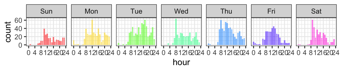
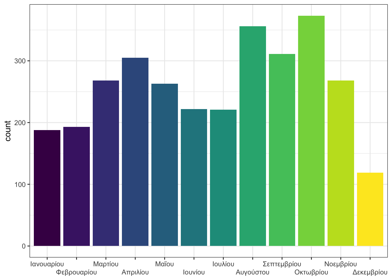
A nice side-effect of using the lubridate function to get days of the week or months of the year is that the results are an ordered factor, so display correctly in a plot. Let’s display the months in Greek (if that’s available on your system).