5 Data Relations
Intended Learning Outcomes
5.1 Functions used
- built-in (you can always use these without loading any packages)
- tidyverse (you can use all these with
library(tidyverse))- readr::
write_csv(),read_csv() - dplyr::
left_join(),right_join(),inner_join(),full_join(),semi_join(),anti_join(),bind_rows(),bind_cols(),intersect(),union(),setdiff(),mutate() - tibble::
tibble(),as_tibble() - purrr::
map_df() - stringr::
str_replace_all()
- readr::
5.2 Set-up
- Open your
ADS-2026project - Download the Data transformation cheatsheet
- Create a new quarto file called
05-relations.qmd - Update the YAML header
- Replace the setup chunk with the one below
5.3 Loading data
The data you want to report on or visualise are often in more than one file (or more than one tab of an excel file or googlesheet). You might need to join up a table of patient information with a table of visits, or combine the monthly social media reports across several months.
For this demo, rather than loading in data, we’ll create two small data tables from scratch using the tibble() function.
patients has id, city and postcode for five patients 1-5.
-
1:5will fill the variableidwith all integers between 1 and 5. -
cityandcodeboth use thec()function to enter multiple strings. Note that each entry is contained within its own quotation marks, apart from missing data, which is recorded asNA. - When entering data like this, it’s important that the order of each variable matches up. So number 1 will correspond to “Port Ellen” and “PA42 7DU”.
| id | city | postcode |
|---|---|---|
| 1 | Port Ellen | PA42 7DU |
| 2 | Dufftown | AB55 4DH |
| 3 | NA | NA |
| 4 | Aberlour | AB38 7RY |
| 5 | Tobermory | PA75 6NR |
visits has patient id and the number of visits to the GP in the last year. Some patients from the previous table have no visits, some have more than one visit, and some are not in the patients table.
| id | visits |
|---|---|
| 2 | 2 |
| 3 | 1 |
| 4 | 4 |
| 4 | 0 |
| 5 | 9 |
| 5 | 11 |
| 6 | 5 |
| 6 | 0 |
| 7 | 3 |
Insert a new code chunk and create the objects patients and visits.
5.4 Mutating Joins
Mutating joins act like the dplyr::mutate() function in that they add new columns to one table based on values in another table. (We’ll learn more about the mutate() function in Chapter 8).)
All the mutating joins have this basic syntax:
****_join(x, y, by = NULL, suffix = c(".x", ".y"))
-
x= the first (left) table -
y= the second (right) table -
by= what columns to match on. If you leave this blank, it will match on all columns with the same names in the two tables. -
suffix= if columns have the same name in the two tables, but you aren’t joining by them, they get a suffix to make them unambiguous. This defaults to “.x” and “.y”, but you can change it to something more meaningful.
You can leave out the by argument if you’re matching on all of the columns with the same name, but it’s good practice to always specify it so your code is robust to changes in the loaded data.
For each of the joins below, run the code and inspect the object it creates and make a note of three things in your Quarto document alongside each bit of code:
- Does the resulting object have more or less observations than the original tables?
- Does the resulting object have more or less variables than the original tables?
- Does the resulting object have any NAs?
5.4.1 left_join()
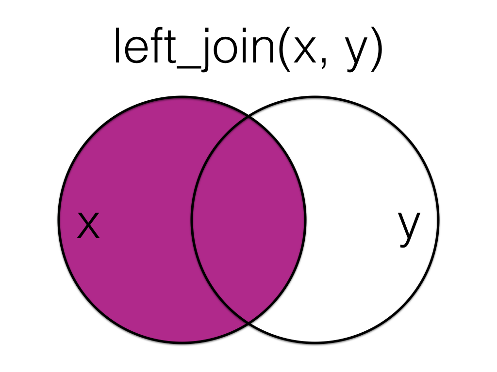
A left_join keeps all the data from the first (left) table and adds anything that matches from the second (right) table. If the right table has more than one match for a row in the left table, there will be more than one row in the joined table (see ids 4 and 5).
| id | city | postcode | visits |
|---|---|---|---|
| 1 | Port Ellen | PA42 7DU | NA |
| 2 | Dufftown | AB55 4DH | 2 |
| 3 | NA | NA | 1 |
| 4 | Aberlour | AB38 7RY | 4 |
| 4 | Aberlour | AB38 7RY | 0 |
| 5 | Tobermory | PA75 6NR | 9 |
| 5 | Tobermory | PA75 6NR | 11 |
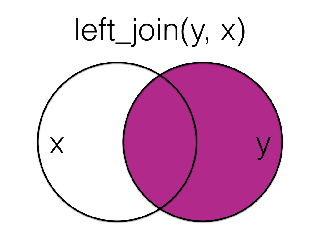
The order you specify the tables matters, in the below code we have reversed the order and so the result is all rows from the visits table joined to any matching rows from the patients table.
5.4.2 right_join()
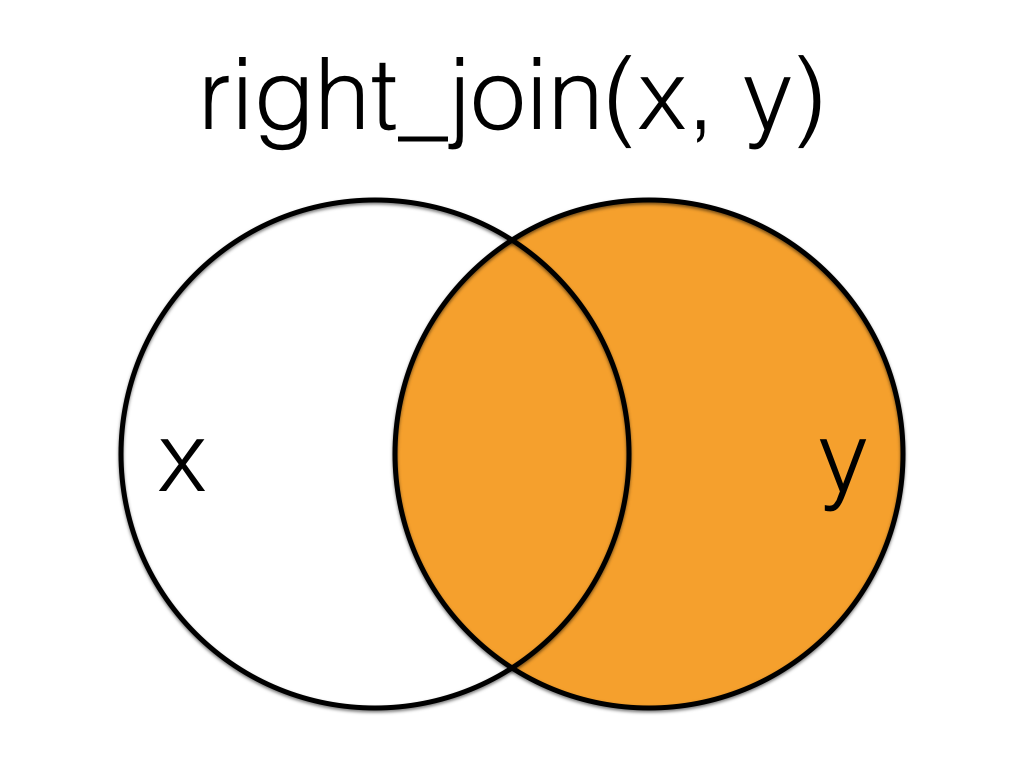
A right_join keeps all the data from the second (right) table and joins anything that matches from the first (left) table.
| id | city | postcode | visits |
|---|---|---|---|
| 2 | Dufftown | AB55 4DH | 2 |
| 3 | NA | NA | 1 |
| 4 | Aberlour | AB38 7RY | 4 |
| 4 | Aberlour | AB38 7RY | 0 |
| 5 | Tobermory | PA75 6NR | 9 |
| 5 | Tobermory | PA75 6NR | 11 |
| 6 | NA | NA | 5 |
| 6 | NA | NA | 0 |
| 7 | NA | NA | 3 |
This table has the same information as left_join(visits, patients, by = "id"), but the columns are in a different order (left table, then right table).
5.4.3 inner_join()
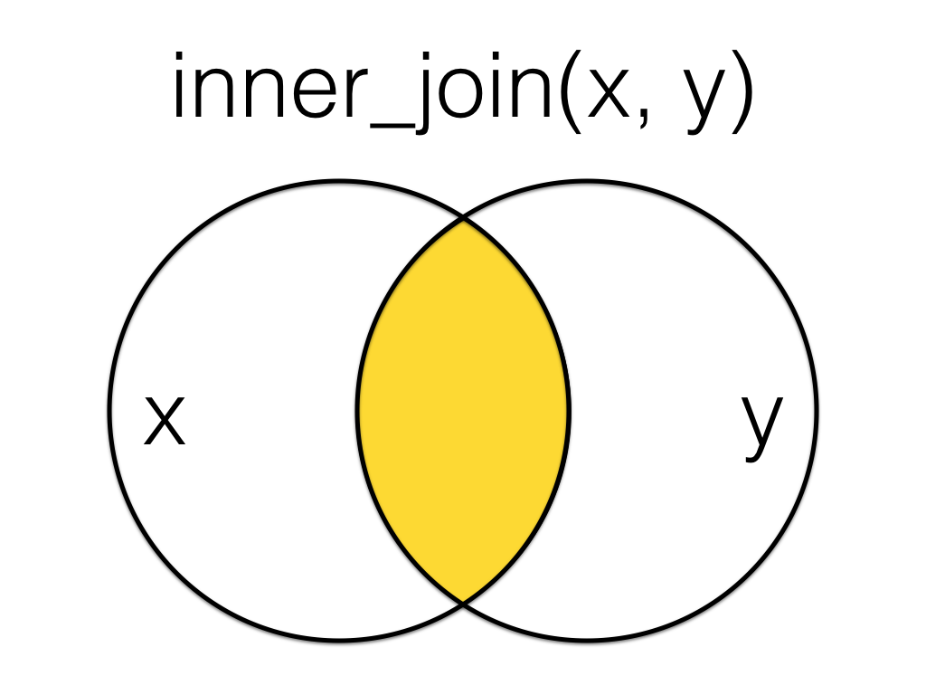
An inner_join returns all the rows that have a match in both tables. Changing the order of the tables will change the order of the columns, but not which rows are kept.
5.4.4 full_join()
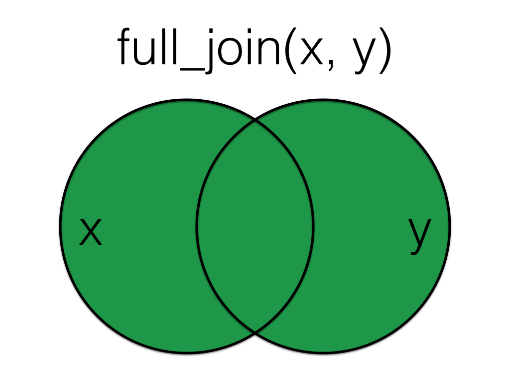
A full_join lets you join up rows in two tables while keeping all of the information from both tables. If a row doesn’t have a match in the other table, the other table’s column values are set to NA.
| id | city | postcode | visits |
|---|---|---|---|
| 1 | Port Ellen | PA42 7DU | NA |
| 2 | Dufftown | AB55 4DH | 2 |
| 3 | NA | NA | 1 |
| 4 | Aberlour | AB38 7RY | 4 |
| 4 | Aberlour | AB38 7RY | 0 |
| 5 | Tobermory | PA75 6NR | 9 |
| 5 | Tobermory | PA75 6NR | 11 |
| 6 | NA | NA | 5 |
| 6 | NA | NA | 0 |
| 7 | NA | NA | 3 |
- You have two datasets: people registered with a GP practice (registrations) and people who received a flu jab (jabs). You only want people who appear in both datasets, because you are analysing outcomes for those registered and vaccinated. Which should you use?
inner_join(registrations, jabs, by = "nhs_number") returns only the people whose NHS number appears in both datasets. This is appropriate when you want to analyse the subset who are both registered and vaccinated, excluding anyone who is only in one list.
- A local authority has two separate lists of households receiving support: one for fuel poverty payments (fuel_support) and one for disability-related housing adaptations (adaptations). You want a combined dataset that includes everyone in either list, keeping both sets of variables and using NA where a household is only in one list. Which should you use?
full_join(fuel_support, adaptations, by = "household_id") keeps all households from both lists and combines the variables, filling unmatched values with NA. This is the correct choice when you want a complete picture of anyone receiving either type of support, not just the overlap.
- You have a table of all NHS boards with their deprivation quintile and population (boards), and a second table with the number of people who attended a new vaccination clinic (attendances). You want a dataset that keeps every NHS board, and adds the attendance numbers where available, showing NA for boards with no recorded attendances. Which should you use?
left_join(boards, attendances, by = "board_id") keeps all rows from boards and adds attendance information where a match exists. NHS boards with no recorded attendances remain in the dataset with NA in the attendance columns, which is what you need for comparing service uptake across all boards.
5.5 Filtering Joins
Filtering joins act like the dplyr::filter() function in that they keep and remove rows from the data in one table based on the values in another table. The result of a filtering join will only contain rows from the left table and have the same number or fewer rows than the left table. We’ll learn more about the filter() function in Chapter 9.
5.5.1 semi_join()
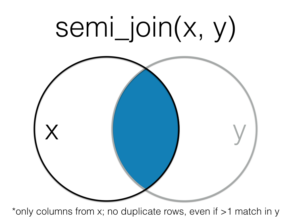
A semi_join returns all rows from the left table where there are matching values in the right table, keeping just columns from the left table.
| id | city | postcode |
|---|---|---|
| 2 | Dufftown | AB55 4DH |
| 3 | NA | NA |
| 4 | Aberlour | AB38 7RY |
| 5 | Tobermory | PA75 6NR |
Unlike an inner join, a semi join will never duplicate the rows in the left table if there is more than one matching row in the right table.

Order matters in a semi join.
5.5.2 anti_join()
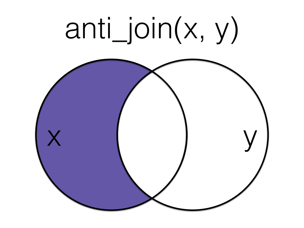
An anti_join return all rows from the left table where there are not matching values in the right table, keeping just columns from the left table.
| id | city | postcode |
|---|---|---|
| 1 | Port Ellen | PA42 7DU |
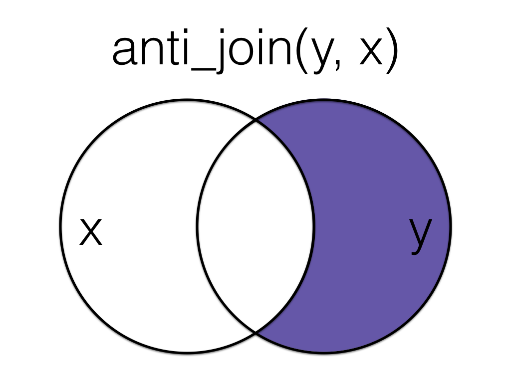
Order matters in an anti join.
- You have a dataset of people discharged from hospital (discharges) and a dataset of people who received a follow up call within 72 hours (followups). You want a list of people who were discharged but did not receive the follow up call. Which should you use?
anti_join(discharges, followups, by = "patient_id") keeps the rows in discharges that do not have a matching patient_id in followups. This directly returns the list of discharged patients who did not receive a follow up call within the specified window.
- You have a dataset of all patients referred to a specialist service (referrals) and a dataset containing those who meet an eligibility criterion after triage (eligible). You want to keep only the referrals that are eligible, but you do not need any additional columns from eligible. Which should you use?
semi_join(referrals, eligible, by = "referral_id") filters referrals to only those rows with a matching referral_id in eligible, but it does not bring in any columns from eligible. This is appropriate when you want an eligibility filter rather than a merged dataset.
5.6 Multiple joins
The ****_join() functions are all two-table verbs, that is, you can only join together two tables at a time. However, you may often need to join together multiple tables. To do so, you simply need to add on additional joins. You can do this by creating an intermediate object or more efficiently by using a pipe.
At every stage of any analysis you should check your output to ensure that what you created is what you intended to create, but this is particularly true of joins. You should be familiar enough with your data through routine checks using functions like glimpse(), str(), and summary() to have a rough idea of what the join should result in. At the very least, you should know whether the joined object should result in more or fewer variables and observations and whether there should be any NAs.
If you have a multi-line join like in the above piped example, build up the code and check the output at each stage.
5.7 Binding Joins
Binding joins bind one table to another by adding their rows or columns together.
5.7.1 bind_rows()
You can combine the rows of two tables with bind_rows.
Here we’ll add patient data for patients 6-9 and bind that to the original patient table.
| id | city | postcode |
|---|---|---|
| 1 | Port Ellen | PA42 7DU |
| 2 | Dufftown | AB55 4DH |
| 3 | NA | NA |
| 4 | Aberlour | AB38 7RY |
| 5 | Tobermory | PA75 6NR |
| 6 | Falkirk | FK1 4RS |
| 7 | Ardbeg | PA42 7EA |
| 8 | Doogal | G81 4SJ |
| 9 | Kirkwall | KW15 1SE |
The columns just have to have the same names, they don’t have to be in the same order. Any columns that differ between the two tables will just have NA values for entries from the other table.
If a row is duplicated between the two tables (like id 5 below), the row will also be duplicated in the resulting table. If your tables have the exact same columns, you can use union() (see Section 5.8.2) to avoid duplicates.
| id | city | postcode | new |
|---|---|---|---|
| 1 | Port Ellen | PA42 7DU | NA |
| 2 | Dufftown | AB55 4DH | NA |
| 3 | NA | NA | NA |
| 4 | Aberlour | AB38 7RY | NA |
| 5 | Tobermory | PA75 6NR | NA |
| 5 | Tobermory | PA75 6NR | 1 |
| 6 | Falkirk | FK1 4RS | 2 |
| 7 | Ardbeg | PA42 7EA | 3 |
| 8 | Doogal | G81 4SJ | 4 |
| 9 | Kirkwall | KW15 1SE | 5 |
5.7.2 bind_cols()
You can merge two tables with the same number of rows using bind_cols. This is only useful if the two tables have the same number of rows in the exact same order.
| id | city | postcode | smoker |
|---|---|---|---|
| 1 | Port Ellen | PA42 7DU | no |
| 2 | Dufftown | AB55 4DH | no |
| 3 | NA | NA | yes |
| 4 | Aberlour | AB38 7RY | yes |
| 5 | Tobermory | PA75 6NR | yes |
The only advantage of bind_cols() over a mutating join is when the tables don’t have any IDs to join by and you have to rely solely on their order. Otherwise, you should use a mutating join (all four mutating joins result in the same output when all rows in each table have exactly one match in the other table).
5.7.3 Importing multiple files
If you need to import and bind a whole folder full of files that have the same structure, get a list of all the files you want to combine. It’s easiest if they’re all in the same directory, although you can use a pattern to select the files you want if they have a systematic naming structure.
First, save the two patient tables to CSV files. The dir.create() function makes a folder called “data”. The showWarnings = FALSE argument means that you won’t get a warning if the folder already exists, it just won’t do anything.
Next, retrieve a list of all file names in the data folder that contain the string “patients”
[1] "data/patients1.csv" "data/patients2.csv"Next, we’ll iterate over this list to read in the data from each file. Whilst this won’t be something we cover in detail in the core resources of this course, iteration is an important concept to know about. Iteration is where you perform the same task on multiple different inputs. As a general rule of thumb, if you find yourself copying and pasting the same thing more than twice, there’s a more efficient and less error-prone way to do it, although these functions do typically require a stronger grasp of programming.
The purrr::map_df() maps a function to a list and returns a data frame (table) of the results.
-
.xis the list of file paths -
.fspecifies the function to map to each of those file paths. - The resulting object
all_fileswill be a data frame that combines all the files together, similar to if you had imported them separately and then usedbind_rows().
If all of your data files have the exact same structure (i.e., the same number of columns with the same names), you can just use read_csv() and set the file argument to a vector of the file names. However, the pattern above is safer if you might have a file with an extra or missing column.
5.8 Set Operations
Set operations compare two tables and return rows that match (intersect), are in either table (union), or are in one table but not the other (setdiff).
5.8.1 intersect()
dplyr::intersect() returns all rows in two tables that match exactly. The columns don’t have to be in the same order, but they have to have the same names.
| id | city | postcode |
|---|---|---|
| 5 | Tobermory | PA75 6NR |
If you’ve forgotten to load dplyr or the tidyverse, base R also has a base::intersect() function that doesn’t work like dplyr::intersect(). The error message can be confusing and looks something like this:
5.8.2 union()
dplyr::union() returns all the rows from both tables, removing duplicate rows, unlike bind_rows().
| id | city | postcode |
|---|---|---|
| 1 | Port Ellen | PA42 7DU |
| 2 | Dufftown | AB55 4DH |
| 3 | NA | NA |
| 4 | Aberlour | AB38 7RY |
| 5 | Tobermory | PA75 6NR |
| 6 | Falkirk | FK1 4RS |
| 7 | Ardbeg | PA42 7EA |
| 8 | Doogal | G81 4SJ |
| 9 | Kirkwall | KW15 1SE |
If you’ve forgotten to load dplyr or the tidyverse, base R also has a base::union() function. You usually won’t get an error message, but the output won’t be what you expect.
[[1]]
[1] 1 2 3 4 5

[[2]]
[1] "Port Ellen" "Dufftown"   NA           "Aberlour"   "Tobermory"

[[3]]
[1] "PA42 7DU" "AB55 4DH" NA         "AB38 7RY" "PA75 6NR"

[[4]]
[1] 5 6 7 8 9

[[5]]
[1] "PA75 6NR" "FK1 4RS"  "PA42 7EA" "G81 4SJ"  "KW15 1SE"

[[6]]
[1] "Tobermory" "Falkirk"   "Ardbeg"    "Doogal"    "Kirkwall"
5.8.3 setdiff()
dplyr::setdiff returns rows that are in the first table, but not in the second table.
| id | city | postcode |
|---|---|---|
| 1 | Port Ellen | PA42 7DU |
| 2 | Dufftown | AB55 4DH |
| 3 | NA | NA |
| 4 | Aberlour | AB38 7RY |
Order matters for setdiff.
| id | postcode | city |
|---|---|---|
| 6 | FK1 4RS | Falkirk |
| 7 | PA42 7EA | Ardbeg |
| 8 | G81 4SJ | Doogal |
| 9 | KW15 1SE | Kirkwall |
If you’ve forgotten to load dplyr or the tidyverse, base R also has a base::setdiff() function. You usually won’t get an error message, but the output might not be what you expect because base::setdiff() expects columns to be in the same order, so id 5 here registers as different between the two tables.
- Two surveys used the same questions and columns, one run in 2023 (survey_2023) and one in 2024 (survey_2024). You want one dataset with all responses from both years, keeping duplicates if the same respondent appears twice. Which should you use?
bind_rows() stacks two data frames on top of each other, so you get all responses from 2023 and 2024 in one long dataset. It keeps duplicates by default, which is appropriate if the same respondent appears in both years and you want both records retained.
- You have two extracts of the same equality register (register_a, register_b) with identical columns. Some rows are exact duplicates across the two extracts. You want a combined dataset that removes exact duplicate rows. Which should you use?
union() combines the rows from both extracts but drops exact duplicate rows, so repeated entries across register_a and register_b are removed. This is useful when the columns match and you want a deduplicated combined register without having to identify duplicates manually.
- You have a master list of staff IDs expected in an annual pay gap analysis (master_staff) and a list of staff IDs present in the HR export you received (hr_export). You want to identify staff who are in the master list but missing from the export. Which should you use?
setdiff(master_staff, hr_export) returns the IDs that are in master_staff but not in hr_export, which is exactly what you want for a missingness check. Order matters, so reversing the inputs would answer a different question (who is in the export but not the master list).
- You have a dataset with one row per patient (patients) and a separate table with model predictions in the same row order (preds), with no shared identifier. You want to add the prediction column to the patients dataset. Which should you use?
bind_cols() adds columns side by side, which is the right choice when patients and preds have the same number of rows and are already aligned in the same row order. Because there is no shared identifier to join on, a join would be inappropriate and could silently misalign records if the order differs.
5.9 Conflicting variable types
As we covered in Chapter 4, when you import or create data, R will do its best to set each column to an appropriate data type. However, sometimes it gets it wrong or sometimes there’s something in the way the data has been encoded in the original spreadsheet that causes the data type to be different than expected. When joining datasets by common columns, it’s important that not only are the variable names identical, but the data type of those variables is identical.
Let’s recreate our new_patients dataset but this time, we’ll specify that id is a character variable.
tibble [5 × 3] (S3: tbl_df/tbl/data.frame)
 $ id      : chr [1:5] "5" "6" "7" "8" ...
 $ postcode: chr [1:5] "PA75 6NR" "FK1 4RS" "PA42 7EA" "G81 4SJ" ...
 $ city    : chr [1:5] "Tobermory" "Falkirk" "Ardbeg" "Doogal" ...
If you try to join this dataset to any of the other datasets where id is stored as a numeric variable, it will produce an error.
Joining with `by = join_by(id, city, postcode)`Error in `inner_join()`:
! Can't join `x$id` with `y$id` due to incompatible types.
ℹ `x$id` is a <integer>.
ℹ `y$id` is a <character>.The same goes for bind_rows():
Error in `bind_rows()`:
! Can't combine `..1$id` <integer> and `..2$id` <character>.
As alternative method to change variable types from what we showed you in Chapter 4 is to use the as.*** functions. If you type as. into a code chunk, you will see that there are a huge number of these functions for transforming variables and datasets to different types. Exactly which one you need will depend on the data you have, but a few commonly used ones are:
-
as.numeric()- convert a variable to numeric. Useful for when you have a variable of real numbers that have been encoded as character. Any values that can’t be turned into numbers (e.g., if you have the word “missing” in cells that you have no data for), will be returned asNA. -
as.factor()- convert a variable to a factor. You can set the factor levels and labels manually, or use the default order (alphabetical). -
as.character()- convert a variable to character data. -
as_tibble()andas.data.frame()- convert a list object (not a variable) to a tibble or a data frame (two different table formats). This isn’t actually relevant to what we’re discussing here, but it’s a useful one to be aware of because sometimes you’ll run into issues where you get an error that specifically requests your data is a tibble or data frame type and you can use this function to overwrite your object.
To use these functions on a variable we can use mutate() to overwrite the variable with that variable as the new data type:
Once you’ve done this, the joins will now work:
5.10 Advanced
If you would like to go beyond what we’ve covered in this chapter, we recommend the following Advanced appendices that are related to this chapter:
- Advanced: Data Import (Appendix C)
- Advanced: Data Types (Appendix D)
5.11 Peer Coding Exercises
If you are enrolled on PSYCH1012 Applied Data Skills, do not do these exercises until the Tuesday workshop.
For each exercise, you will work in a pair programming team. Pair programming is when two people work on the same code with distinct, rotating roles:
The Driver operates the keyboard, implements the next small step, narrates what they are doing.
The Navigator reviews in real time, thinks ahead, checks naming, design, and help pages, and catches mistakes and typos.
You should work in short cycles (5 to 10 minutes or two or three tasks), then switch roles.
There are no solutions provided for the pair programming activities. Everything you need is in this chapter of the book so use the search function and work together to solve any problems.
Decide who is going to start as the Driver and Navigator. Remember to switch every so often. The Navigator will find it helpful to have a copy of these instructions open and read the next step to the Driver.
Open RStudio, ensure the environment is clear, and restart R.
Create a new quarto document and save it as ads-week6-joins.qmd
In a new code chunk, load the tidyverse.
5.11.1 Grade data
The University of Glasgow’s Schedule A grading scheme uses a 22-point alphanumeric scale (there’s more information in your summative report assessment information sheet). Each alphanumeric grade (e.g., B2) has an underlying numeric Grade Point (e.g., 16).
Often when we’re working with student grades they are provided to us in only one of these forms, but we need to be able to go between the two. For example, we need the numeric form in order to be able to calculate descriptive statistics about the mean grade, but we need the alphanumeric form to release to student records.
Download grade_data.csv, grade_data2.csv and scheduleA.csv into your data folder.
Read each file into R and store them as grades1, grades2, and schedule.
5.11.2 Matching the variable types
At UofG, all students are given a GUID, a numeric ID number. However, that ID number is also then combined with the first letter from your surname to create your username that is used with your email address. For example, if your ID is 1234567 and your surname is Nordmann, your username would be 1234567n. From a data wrangling perspective this is very annoying because the numeric ID will be stored as numeric data, but the username will be stored as character because of the letter at the end. grades1 has a numeric id whilst grades2 has the additional letter. In order to join these datasets, we need to standardise the variables.
First, remove the letter character from
idusing the functionstringr::str_replace_all(), which replaces text that matches a pattern. Here, we’re using the pattern"[a-z]", which matches all lowercase letters a through z, and replacing them with"". See the help for?about_search_regexfor more info about how to set patterns (these can get really complex).Now, transform the data type of
idso that it matches the data type ingrades2.
5.11.3 Complete records
In this example, we want to join the grade data to schedule A so that each student with a grade has both the grade and the grade point. But we also want a complete record of all students on the course, so students with missing grades should still be included in the data.
- Join
grades1andscheduleAand store this table in an object namedexam_all. - Do the same for
grades2and save it inessay_all. - Both
exam_allandessay_allshould have 100 observations of 4 variables.
You want to keep all of the data from grade_data1 and grade_data2, but you only want the alphanumeric grades from schedule for the Grade Point values that exist in grades. E.g., if no-one was awarded an F1, your final dataset shouldn’t have that in it.
5.11.4 Missing data
Alternatively, you may wish to have a dataset that only contains data for students who submitted each assessment and have a grade. First, run summary() on both exam_all and essay_all.
- How many exam grades are missing?
- How many essay grades are missing?
- Now, create an object
exam_gradesthat joins togethergrades1andschedule, but this time the resulting object should only contain data from students who have a grade. Do the same but forgrades2and store it inessay_grades.
Before you do this, given what you know about how many data points are missing in each data set:
- How many observations should
exam_gradeshave? - How many observations should
essay_gradeshave?
It’s worth noting that in reality you wouldn’t actually go back to the raw data and do another join to get this dataset, you could just remove all the missing response by adding |> drop_na() to exam_all and essay_all. However, for the purposes of teaching joins, we’ll do it this slightly artificial way.
Now, create a dataset
completesthat joins the grades for students who have a grade for both the essay and the exam. Because bothexam_gradesandessay_gradeshave the variablesAssessment,PointsandGradesthat are named the same, but have different data, you should amend the suffix so that the resulting variables are namedPoints_examandPoints_essayetc. You may need to consult the help documentation to see an example to figure this out.Clean up the file with
select()and only keep the variablesid,Grade_exam, andGrade_essay
- How many students have a grade for both the exam and the essay?
- Now create a dataset
no_essaythat contains students that have a grade for the exam, but not the essay.
- How many students have a grade for the exam but not the essay?
Finally, now make a dataset
no_examthat contains students have have a grade for the essay but not the examHow many students have a grade for the exam but not the essay?
5.12 Glossary
| term | definition |
|---|---|
| base-r | The set of R functions that come with a basic installation of R, before you add external packages. |
| binding-joins | Joins that bind one table to another by adding their rows or columns together. |
| character | A data type representing strings of text. |
| factor | A data type where a specific set of values are stored with labels; An explanatory variable manipulated by the experimenter |
| filtering-joins | Joins that act like the dplyr::filter() function in that they remove rows from the data in one table based on the values in another table. |
| iteration | Repeating a process or function |
| mutating-joins | Joins that act like the dplyr::mutate() function in that they add new columns to one table based on values in another table. |
| numeric | A data type representing a real decimal number or integer. |
| set-operations | Functions that compare two tables and return rows that match (intersect), are in either table (union), or are in one table but not the other (setdiff). |
5.13 Further resources
- Data transformation cheatsheet
- Chapter 19: Joins in R for Data Science
- Chapter 26: Iteration in R for Data Science.
- purrr cheatsheet