15 N

15.1 NA

A missing value that is "Not Available"

You can use NA to represent missing values in a vector. Use the function is.na() to check if values are missing.

values <- c(1,4,NA,3,4)
is.na(values)
#> [1] FALSE FALSE  TRUE FALSE FALSE

If the results of a calculation like mean() or sd() is NA, this usually means that you have some missing values in your vector. You can remove NA values using na.rm = TRUE in many functions.

mean(values)
#> [1] NA
mean(values, na.rm = TRUE)
#> [1] 3

Dealing with missing values when calculating correlations is a little trickier.

dat <- tribble(
  ~x, ~y, ~z,
   1,  3, NA, # x-y included when p.c.o
   2,  1,  4, 
   3,  5,  3,
   4,  1,  2,
  NA,  5,  1  # y-z included when p.c.o
)


# uses only rows 2:4 for all correlations
cor(dat, use = "complete.obs")
#>    x y  z
#> x  1 0 -1
#> y  0 1  0
#> z -1 0  1

# uses rows 1:4 for x-y, 2:5 for y-z, and 2:4 for x-z
cor(dat, use = "pairwise.complete.obs")
#>          x          y          z
#> x  1.00000 -0.1348400 -1.0000000
#> y -0.13484  1.0000000 -0.4472136
#> z -1.00000 -0.4472136  1.0000000

You can filter a table down to only rows with no NA values using na.omit().

complete_dat <- na.omit(dat)

x	y	z
2	1	4
3	5	3
4	1	2

15.2 NaN

An impossible number that is "Not a number"

In R impossible numbers are represented with the symbol NaN. Use the function is.nan() to check if values are impossible numbers.

value <- 0/0
value
#> [1] NaN
is.nan(value)
#> [1] TRUE

15.3 NHST

Null Hypothesis Signficance Testing

15.4 nominal

Categorical variables that don't have an inherent order, such as types of animal.

15.5 normal distribution

A symmetric distribution of data where values near the centre are most probable.

A normal distribution is characterised by its mean and standard deviation. You can sample numbers from a simulated normal distribution with the function rnorm().

# sample 1 million numbers from a normal distribution with 
# a mean of 0 and a standard deviation of 1
x <- rnorm(1000000, mean = 0, sd = 1)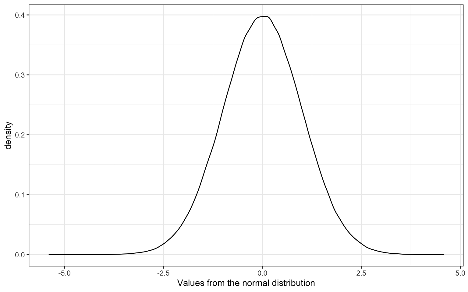

Figure 15.1: Normal Distribution

About 68% of the values are within 1 SD of the mean.

# proportion between -1 and 1
mean(x > -1 & x < 1)
#> [1] 0.682617

About 95% of the values are within 2 SDs of the mean.

# proportion between -2 and 2
mean(x > -2 & x < 2)
#> [1] 0.954465

15.6 null effect

An outcome that does not show an otherwise expected effect.

A null effect could be a difference of 0 between two groups, or a chance value, such as 50% in a two-alternative forced choice task.

15.7 null hypothesis

The hypothesis that an observed difference between groups or from a specific value is due to chance alone.

The null hypothesis is also commonly referred to as H0. This is contrasted with H1, the alternate hypothesis in a null hypothesis significance testing (NHST) framework.

15.8 numeric

A data type representing a real decimal number or integer.

The integer and double data types are numeric.

You can check if a variable is numeric using the function is.numeric and you can convert a variable to its numeric representation using the function as.numeric.

is.numeric(2.4)
#> [1] TRUE

is.numeric(2L)
#> [1] TRUE

# complex numbers are not numeric 
is.numeric(2i)
#> [1] FALSE

is.numeric("A")
#> [1] FALSE

# numbers represented as strings are not numeric
is.numeric("3")
#> [1] FALSE

as.numeric(2.4)
#> [1] 2.4

as.numeric(2L)
#> [1] 2

# the imaginary part of complex numbers is discarded when converting to numeric
as.numeric(3+2i)
#> Warning: imaginary parts discarded in coercion
#> [1] 3

# strings that do not represent numbers are converted to NA
as.numeric("A")
#> Warning: NAs introduced by coercion
#> [1] NA

# numbers represented as strings can be convertd to their numeric version
as.numeric("3")
#> [1] 3