19 R
19.1 R markdown
The R-specific version of markdown: a way to specify formatting, such as headers, paragraphs, lists, bolding, and links, as well as code blocks and inline code.
More...
An R markdown file starts with a YAML header that usually contains the title, author, and output type.
---
title: "Analysis Plan Template"
author: "School of Psychology, University of Glasgow"
output: html_document
---
The rest of the file is a mix of markdown and code chunks. Here is an example of two section titles. The first section has an r chunk for loading the packages and the second section has a list of steps.
## Packages used

```{r setup, include = FALSE}
# every time you add a new package, include it in this section
library(tidyverse)
```

## Data Processing

1. load in packages
2. load in dataset
3. Wrangle data into appropriate format for analysis and checks. You might want to reshape the data or combine different values to make a new variable.
Resources:
19.2 R-squared
A statistic that represents the proportion of the variance for a dependent variable explained by the predictor variable(s) in a linear model.
More...
Let's simulate some data:
# simulate some data
set.seed(8675309)

n <- 100
intercept <- 10
effect <- 0.5
error_sd <- 2

dat <- tibble::tibble(
  predictor = rnorm(n, 0, 1),
  error = rnorm(n, 0, error_sd),
  dv = intercept + (effect * predictor) + error
)
Analyse the data with a linear model and use the summary() function to view the R-squared values.
model <- lm(dv ~ predictor, dat)
summary(model)
#>
#> Call:
#> lm(formula = dv ~ predictor, data = dat)
#>
#> Residuals:
#>     Min      1Q  Median      3Q     Max
#> -5.0692 -1.4106  0.2447  1.4562  3.9263
#>
#> Coefficients:
#>             Estimate Std. Error t value Pr(>|t|)
#> (Intercept)   9.8913     0.1991  49.677  < 2e-16 ***
#> predictor     0.6361     0.2150   2.958  0.00388 **
#> ---
#> Signif. codes:  0 '***' 0.001 '**' 0.01 '*' 0.05 '.' 0.1 ' ' 1
#>
#> Residual standard error: 1.988 on 98 degrees of freedom
#> Multiple R-squared:  0.08198,    Adjusted R-squared:  0.07261
#> F-statistic: 8.752 on 1 and 98 DF,  p-value: 0.003877
Adjusted R-squared is a modified version of R-squared adjusted for the number of predictors in the model. You can extract the R-squared and adjusted R-squared values from the model summary.
19.3 random effect
An effect associated with an individual sampling unit, usually represented by an offset from a fixed effect.
Example: If the grand mean response time in a population is 600 milliseconds, that number represents the typical value. The mean response time for an individual subject \(s\) can be represented as an offset (deviation) from that value. For example, if subject \(s\) has a mean reaction time of 650 ms, that would imply a random effect for that subject of +50 ms.
Unlike fixed effects, we expect the underlying random effects to change from experiment to experiment as the sampling units (e.g., subjects) change.
In a mixed effects model, you can get a table of just the random effects with the code below:
model <- afex::lmer(
  rating ~ rater_age * face_age + # fixed effects
  (1 | rater_id) + (1 | face_id), # random effects
  data = faux::fr4
)

broom.mixed::tidy(model, effects = "ran_pars")| effect | group | term | estimate |
|---|---|---|---|
| ran_pars | face_id | sd__(Intercept) | 0.6040734 |
| ran_pars | rater_id | sd__(Intercept) | 0.9144817 |
| ran_pars | Residual | sd__Observation | 1.0434014 |
19.4 random factor
A factor whose levels are taken to represent a proper subset of a population of interest, typically because the observed levels are the result of sampling.
If you perform a study where the population of interest is "undergraduates at the University of Glasgow", you are very unlikely to obtain data from all approximately 20,000 undergraduate students. Instead, you would likely obtain a (hopefully random) sample of undergraduates, with each undergraduate forming a single 'level' of the 'subject' factor. By treating 'subject' as random rather than fixed in your analysis, you will obtain parameter estimates that are closer to the true population values.
Random factors are usually contrasted with fixed factors, whose levels are assumed to represent all the levels of interest in a population.
19.5 random seed
A value used to set the initial state of a random number generator.
Random seeds are used in random number generation. Each time you generate a random number, the number you get depends on the state of the underlying random number generator. If you set this state to a known value, you will get the same random numbers in the same order.
Random seeds are used to make processes that involve random values reproducible. In R, you can set a random seed using the set.seed() function. If you put set.seed() at the start of your script, you will get the same output every time.
19.6 reactivity
Changes in a Shiny app that occur in response to user input.
19.7 README
A text file in the base directory of a project that describes the project.
A README is a plain text file that contain information you want new users of the project to read first. This commonly contains one or more of the following: configuration or installation instructions, a list of files included with the project, a usage license, citation information, and author contact info.
19.8 relative path
The location of a file in relation to the working directory.
For example, if your working directory is /Users/me/study/ and you want to refer to a file at /Users/me/study/data/faces.csv, the relative path is data/faces.csv. Use ../ to move up one directory.
# the working directory: /Users/me/study/

# read a file inside the wd: /Users/me/study/data/faces.csv
qdat <- readr::read_csv("data/faces.csv")

# read a file outside the wd: /Users/me/other_study/data/exp.csv
xdat <- readr::read_csv("../other_study/data/exp.csv")
Make sure you always use relative paths in an R Markdown document, which automatically sets the working directory to the directory that contains the .Rmd file.
Contrast with absolute path.
19.9 render
To create a file (usually an image or PDF) or widget from source code
In the context of Shiny apps, render usually means to create the HTML to display in a reactive output from code in the server section.
In the context of R Markdown files, knit, render and compile tend to be used interchangeably.
19.10 repeated measures
A dataset has repeated measures if there are multiple measurements taken on the same variable for individual sampling units.
See also multilevel.
19.11 replicability
The extent to which the findings of a study can be repeated with new samples from the same population.
Alternatively, a scientific claim is replicable if it is supported by new data (Errington et al., 2021).
See also reproducibility.
The aim of replicating a study is test the underlying theoretical process, estimate the average effect size, and test whether you can observe the effect independent of the original researchers by recreating a study's methods as closely as possible (Brandt et al., 2014).
There is not a clear definition for a successful replication, but there are some common markers (Errington et al., 2021):
- Is the replication effect in the same direction as the original study?
- Is the replication effect and statistical significance in the same direction as the original study?
- Is the effect size from the original study in the confidence interval of the replication?
- Is the effect size from the replication study in the confidence interval of the original?
- Is the effect size from the replication smaller or equal to the effect size from the original study?
19.12 reprex
A reproducible example that is the smallest, completely self-contained example of your problem or question.
For example, you may have a question about how to figure out how to select rows that contain the value "test" in a certain column, but it isn't working. It's clearer if you can provide a concrete example, but you don't want to have to type out the whole table you're using or all the code that got you to this point in your script.
You can include a very small table with just the basics or a smaller version of your problem. Make comments at each step about what you expect and what you actually got.
More...
Which version is easier for you to figure out the solution?
# this doesn't work
no_test_data <- data %>%
  filter(!str_detect(type, "test"))
# with a minimal example table
data <- tribble(
  ~id, ~type, ~x,
  1, "test", 12,
  2, "testosterone", 15,
  3, "estrogen", 10
)

# this should keep IDs 2 and 3, but removes ID 2
no_test_data <- data %>%
  filter(!str_detect(type, "test"))
One of the big benefits to creating a reprex is that you often solve your own problem while you're trying to break it down to explain to someone else.
If you really want to go down the rabbit hole, you can create a reproducible example using the reprex package from tidyverse.
19.13 reproducibility
The extent to which the findings of a study can be repeated in some other context
Reproducibility can be either with new samples from the same population (replicability) or with the same raw data but analyzed by different researchers or by the same researchers on a different occasion (computational or analytical reproducibility).
19.14 reproducible research
Research that documents all of the steps between raw data and results in a way that can be verified.
19.15 residual
Defined as the deviation of an observation from a model's expected value.
Mathematically, the residual is defined as the observed value minus the model's fitted value for that observation.
More...
For example, the linear model \(\hat{Y_i} = 3 + 2 X_i\) predicts a value of \(\hat{Y}_i = 7\) for \(X_i = 2\). If you happen to have observed \(Y_i = 8\) for observation \(i\), then the residual for that observation would be \(Y_i - \hat{Y}_i = 8 - 7 = 1\).
A related but slightly different notion is error.
For example, below we simulate data for two groups of 50 with means of 100 and 105 (and SDs of 10).
set.seed(8675309) # for reproducibility

group0 <- rnorm(n = 50, mean = 100, sd = 10)
group1 <- rnorm(n = 50, mean = 105, sd = 10)

df <- data.frame(
  dv = c(group0, group1),
  group = rep(0:1, each = 50)
)

model <- lm(dv ~ group, data = df)

summary(model)
#>
#> Call:
#> lm(formula = dv ~ group, data = df)
#>
#> Residuals:
#>      Min       1Q   Median       3Q      Max
#> -25.9878  -7.1828  -0.1015   5.8804  20.1878
#>
#> Coefficients:
#>             Estimate Std. Error t value Pr(>|t|)
#> (Intercept)  101.027      1.319  76.609   <2e-16 ***
#> group          3.992      1.865   2.141   0.0348 *
#> ---
#> Signif. codes:  0 '***' 0.001 '**' 0.01 '*' 0.05 '.' 0.1 ' ' 1
#>
#> Residual standard error: 9.325 on 98 degrees of freedom
#> Multiple R-squared:  0.04467,    Adjusted R-squared:  0.03492
#> F-statistic: 4.582 on 1 and 98 DF,  p-value: 0.03478

model$coefficients
#> (Intercept)       group
#>  101.026918    3.992219
The model above has an intercept of 101 and an effect of group of 4, meaning that the predicted value for group 0 is 101 and the predicted value for group 1 is 105. The difference between these predictions and the observed values is the residual error.
intercept <- model$coefficients[[1]]
effect <- model$coefficients[[2]]

df |>
  mutate(predicted = intercept + effect * group,
         residual = dv - predicted) |>
  group_by(group) |>
slice(1:5) # show 5 from each group| dv | group | predicted | residual |
|---|---|---|---|
| 90.03418 | 0 | 101.0269 | -10.992742 |
| 107.21824 | 0 | 101.0269 | 6.191323 |
| 93.82791 | 0 | 101.0269 | -7.199007 |
| 120.29392 | 0 | 101.0269 | 19.266997 |
| 110.65416 | 0 | 101.0269 | 9.627242 |
| 106.34898 | 1 | 105.0191 | 1.329843 |
| 106.17582 | 1 | 105.0191 | 1.156684 |
| 96.74411 | 1 | 105.0191 | -8.275028 |
| 83.64764 | 1 | 105.0191 | -21.371500 |
| 107.14209 | 1 | 105.0191 | 2.122948 |
19.16 response variable
A variable (in a regression) whose value is assumed to be influenced by one or more predictor variables.
In an experimental context, the response variable is often referred to as the dependent variable.
19.17 right_join
A mutating join that keeps all the data from the second (right) table and joins anything that matches from the first (left) table.
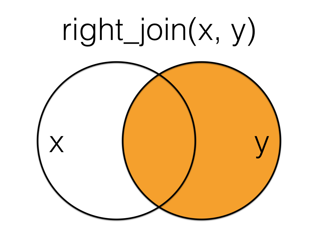
Figure 19.1: Right Join
More...
| Table X | Table Y | ||||||||||||||||||||||||
|---|---|---|---|---|---|---|---|---|---|---|---|---|---|---|---|---|---|---|---|---|---|---|---|---|---|
|
|
If there is no matching data in the left table for a row, the values are set to NA.
# X is the right table
data <- right_join(X, Y, by = "id")| id | x | y |
|---|---|---|
| 2 | B | V |
| 3 | C | W |
| 4 | D | X |
| 5 | E | Y |
| 6 | NA | Z |
Order is important for right joins.
# Y is the right table
data <- right_join(Y, X, by = "id")| id | y | x |
|---|---|---|
| 2 | V | B |
| 3 | W | C |
| 4 | X | D |
| 5 | Y | E |
| 1 | NA | A |
See joins for other types of joins and further resources.
19.18 RStudio
An integrated development environment (IDE) that helps you process R code.
Download RStudio at https://rstudio.com/