5 D

5.1 data frame

A container data type for storing tabular data.

data.frame(
  id = 1:5,
  name = c("Lisa", "Phil", "Helena", "Rachel", "Jack")
)

id	name
1	Lisa
2	Phil
3	Helena
4	Rachel
5	Jack

5.2 data type

The kind of data represented by an object.

• integer (whole numbers like 1L, -10L, 3000L)
• double (numbers like -0.223, 10.324, 1e4)
• character (letters or words like "I love R")
• logical (TRUE or FALSE)
• complex (numbers with real and imaginary parts like 2i)

Integers and doubles are both numeric.

More...

If you want to know what data type a variable is, use the function typeof.

typeof(10)
#> [1] "double"

typeof("10")
#> [1] "character"

typeof(10L)
#> [1] "integer"

typeof(10 == 10)
#> [1] "logical"

typeof(10i)
#> [1] "complex"

5.3 data wrangling

The process of preparing data for visualisation and statistical analysis.

5.4 default value

A value that a function uses for an argument if it is skipped.

For example, mean() has a default value of FALSE for the argument na.rm (don't ignore NA values).

x <- c(1,2,3,NA)
mean(x)
#> [1] NA

So if you leave that argument out, it's the same as setting it to FALSE.

mean(x, na.rm = FALSE)
#> [1] NA

And you have to explicitly set it if you want it to be different.

mean(x, na.rm = TRUE)
#> [1] 2

If an argument does not have a default value, you can't omit it. In the example below, there is no default value for n.

x = rnorm()
#> Error in rnorm(): argument "n" is missing, with no default

TRANSLATED TERM:預設值 任何R函式事先設定的參數數值，編寫程式碼未設定即取用的數值。

請測試以下程式碼：
mean() 的其中一項參數na.rm，預設值是 FALSE(表示計算不忽略NA)。

x <- c(1,2,3,NA)
mean(x)
#> [1] NA

即使寫出參數及預設值，計算結果也是一樣。

mean(x, na.rm = FALSE)
#> [1] NA

更改參數數值，才會得到不同的結果。

mean(x, na.rm = TRUE)
#> [1] 2

如果參數未指定預設值，通常必須手動指定數值。以下例子直接執行會有錯誤，因為參數n沒有預設值。

x = rnorm()
#> Error in rnorm(): argument "n" is missing, with no default

5.5 degrees of freedom

The number of observations that are free to vary to produce a known outcome.

If you run 5 people and ask them their age, and you know the mean age of those 5 people is 20.1, then four of those people can have any age, but the 5th person must have a specific age to maintain the mean of 20.1. The mean age here is the known outcome and four people's age can vary freely, so the degrees of freedom is 4.

You need to know the degrees of freedom (usually abbreviated df) to interpret test statistics like t-values and F-values.

Figure 5.1: How p-values vary depending on the degrees of freedom for specific t-values in a t-test.

自由度 有n個觀察值且已知樣本平均值，不能用已知估計值推測的可變異觀察值個數。

假設你想知道五位同班同學今年幾歲，而你事先知道五人平均20.1歲。樣本平均值是已知的估計值，你只能推測其中一位的真實年齡是20.1歲，但是其他四位回答的年齡可以是任何數值。這個例子的樣本有4個觀察值可自由變異，所以自由度是4。

當你進行統計檢定如t檢定和F檢定，必須要知道正確的自由度(簡寫 df)。

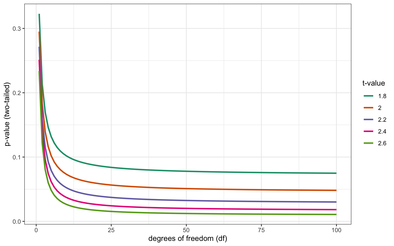
Figure 5.2: How p-values vary depending on the degrees of freedom for specific t-values in a t-test.

中文參考資料：林澤民(2017)。統計學中算變異量為什麼要除以n-1？什麼是「自由度」？

5.6 dependent variable

The target variable that is being analyzed, whose value is assumed to depend on other variables.

You are generally interested in how other variables you have measured impact the dependent variable. For example, if you are testing the effect of stress on anxiety, stress would be your independent variable and anxiety would be the dependent variable. The terms independent/dependent variable are typically used in an experimental context. In the context of regression, the dependent variable is often referred to as the response variable.

依變項 分析程序作用的目標變項之一，數值範圍依賴其他變項的設定。

依變項是測量數值的集合，進行資料分析通常想知道其他變項如何影響測量結果。例如你測量個人感受的壓力如何影響焦慮感，壓力就是你要分析的獨變項，焦慮感就是依變項。實驗研究都稱呼這些變項為獨變項與依變項，迴歸分析則稱呼為反應變項。

5.7 descriptive

Statistics that describe an aspect of data (e.g., mean, median, mode, variance, range)

Contrast with inferential statistics.

5.8 deviation score

A score minus the mean

tibble(
  score = 8:12
) %>%
  mutate(mean = mean(score),
         deviation_score = score - mean)

score	mean	deviation_score
8	10	-2
9	10	-1
10	10	0
11	10	1
12	10	2

5.9 dimension

An axis used to locate or specify a data point in a data structure (e.g., vectors have 1 dimension and data frames have 2: rows and columns)

For example, vectors are 1-dimensional, so you only need one index to specify a value. Data frames and matrices are 2-dimensional, so need two numbers to specify a value. Arrays can have any number of dimensions.

Dimension can also refer to the number of elements in each dimension that an object has, which you can determine with the dim() function (or the length() function for vectors).

More...

The code below arranges the numbers 1 to 12 in data structures with 1, 2 or 3 dimensions and shows how to extract the value 3 from each.

# 1-dimensional vector
v <- 1:12
v
#>  [1]  1  2  3  4  5  6  7  8  9 10 11 12
length(v)
#> [1] 12
v[3] # index
#> [1] 3

# 2-dimensional data frame
df <- data.frame(
  a = 1:6,
  b = 7:12
)
df

a	b
1	7
2	8
3	9
4	10
5	11
6	12

dim(df)
#> [1] 6 2
df[3, 1] # row, column
#> [1] 3

# 2-dimensional matrix
m <- matrix(1:12, nrow = 2)
m
#>      [,1] [,2] [,3] [,4] [,5] [,6]
#> [1,]    1    3    5    7    9   11
#> [2,]    2    4    6    8   10   12
dim(m)
#> [1] 2 6
m[1, 2] # row, column
#> [1] 3

# 3-dimensional array
a <- array(1:12, dim = c(2, 3, 2))
a
#> , , 1
#> 
#>      [,1] [,2] [,3]
#> [1,]    1    3    5
#> [2,]    2    4    6
#> 
#> , , 2
#> 
#>      [,1] [,2] [,3]
#> [1,]    7    9   11
#> [2,]    8   10   12
dim(a)
#> [1] 2 3 2
a[1, 2, 1] # row, column, D3
#> [1] 3

5.10 directory

A collection or "folder" of files on a computer.

In a file path, each directory is separated by forward slashes, e.g., "dir1/dir2/file.Rmd".

Sometimes you need to check if a directory exists and/or make a new directory. For example, a script may save images in a directory called "images" that is in the same directory as the script (so you can use the relative path). Below is code for checking whether that directory exists and making it if it doesn't.

path <- "images"

if (!dir.exists(path)) {
  dir.create(path)
}

5.11 discrete

Data that can only take certain values, such as integers.

Discrete data are not continuous, so it doesn't make sense to have a value that is partway between two values. For example, the number of texts you send per day is discrete; you can't send 12.5 texts. Discrete data can be ordinal or nominal.

5.12 distribution

A probability distribution is way to describe the shape of data.

• normal distribution
• binomial distribution
• Poisson distribution
• uniform distribution

5.13 double brackets

Two pairs of square brackets used to select a single item from a container like a list, data frame, or matrix (e.g., data[[1]]).

data <- data.frame(
  id = 1:3,
  x = c(1.4, 2.3, 8.2)
)

# double brackets return the id column as a vector
data[["id"]] 
#> [1] 1 2 3

See brackets for an explanation of the difference between single and double brackets.

5.14 double

A data type representing a real decimal number.

Examples of doubles are 1, 1.0, -0.01, or 1e4.

5.15 dynamic

Something that can change in response to user actions

For example, in a shiny app, the following code creates dynamic and static elements.

dynamic <- shiny::textOutput("This text can change")
static <- shiny::p("This text cannot change")