6 E
6.1 effect code
A coding scheme for categorical variables that contrasts each group mean with the mean of all the group means.
Also referred to as contrast coding.
6.2 effect size
The difference between the effect in your data and the null effect (usually a chance value)
Effect sizes can be raw (in the same units as the dependent variable) or standardized (in units of standard deviation).
set.seed(8675309) # for simulation reproducibility

dv <- rnorm(n = 1000, mean = 55, sd = 20)
null_value <- 50
raw_effect <- mean(dv) - null_value
std_effect <- raw_effect / sd(dv)
For the example above, we sampled 1000 values from a normal distribution with a mean of 55 and SD of 20. Let's say the DV units here are "percentage points" and the chance value for this example is 50. Therefore, the raw effect is the difference between the mean value and the null value: 4.5 percentage points. The standardized effect is this value, divided by the SD, so the units disappear: 0.2.
Raw effect sizes can be more meaningful in some circumstances (e.g., when multilevel structure makes it hard to define a single SD), while standardized effect sizes can make it easier to compare effects across different experimental designs.
6.3 effect
Some measure of your data, such as the mean value, or the number of standard deviations the mean differs from a chance value.
6.4 element
One item in a vector.
For example, the built-in vector LETTERS contains 26 elements: the uppercase latin letters A through Z. You can select an element from a vector by putting its index in square brackets.
# get the tenth upppercase letter
LETTERS[10]
#> [1] "J"
6.5 element (html)
A unit of HTML, such as a header, paragraph, or image.
In HTML, an element is defined by start and end tags. Labelling parts of HTML content as elements defines how they should be visually displayed (controlled by CSS) and handled by screen readers.
6.6 ellipsis
Three dots (...) representing further unspecified arguments to a function.
When you look up the help for a function, you often see one of the arguments is .... This means that you can supply your own argument names and values here.
More...
For example, the help page for dplyr::mutate() shows a usage of mutate(.data, ...), which means that the first argument is called .data and is the data table you want to mutate, and the second argument is ..., which means that you can add as many new arguments as you want and each one will create a new column with the argument name and value.
# create a data frame with letters and numbers
df <- data.frame(
  number = 1:5,
  letter = LETTERS[1:5]
)

# the mutate function lets you add custom arguments
# like lower and plus_10
mutate(
  .data = df,
  lower = tolower(letter),
  plus_10 = number + 10
)| number | letter | lower | plus_10 |
|---|---|---|---|
| 1 | A | a | 11 |
| 2 | B | b | 12 |
| 3 | C | c | 13 |
| 4 | D | d | 14 |
| 5 | E | e | 15 |
6.7 environment
A data structure that contains R objects such as variables and functions
The Environment pane defaults to showing the contents of the Global Environment. This is where objects defined in the console or interactively running scripts are stored. You can also use the code ls() to list all objects.
When you restart R, the global environment should clear. If it doesn't, go to Global Options... under the Tools menu (⌘,), and uncheck the box that says Restore .RData into workspace at startup. If you keep things around in your workspace, things will get messy, and unexpected things will happen. You should always start with a clear workspace. This also means that you never want to save your workspace when you exit, so set this to Never. The only thing you want to save are your scripts.
You can also use the code rm(list = ls()) or click on the broom icon in the Environment pane to clear the global environment without restarting R.
When you knit an R markdown file, this happens in a new environment, so if any of your code relies on objects you created outside your script, that code will run interactively in R Studio, but will fail when you knit because the objects in the gloabl environment are not available in the knitting environment.
If you start writing your own functions, you need to understand a little about scope and how the environment inside a function is not the same as the global environment. The Environments chapter in Advanced R is a good resource for advanced understanding.
6.8 error term
The term in a model that represents the difference between the actual and predicted values
In the standard regression model
\[Y_i = \beta_0 + \beta_1 X_i + e_i\]
the parameter \(e_i\) represents the error term.
Model formulae typically do not include an explicit error term; it is implicit. For example, the linear model formula below only includes a main effect of group; the intercept and error term are implied.
lm(dv ~ group, data = df)See residual for a concrete example.
6.9 error
The statistical error in a linear model is how much an observation's value differs from the (typically unobserved) true value of a population parameter.
It is closely related to the notion of a residual, except that it reflects deflection from the (usually unknown) true value as opposed to an estimate of the true value. It is usually only possible to know an observation's error if one is dealing with simulated data.
6.10 escape
Include special characters like " inside of a string by prefacing them with a backslash.
When you need to use a character that has a special meaning in R or markdown, you can create the literal version by escaping it with a backslash.
str <- "This prints a \"quote\" and prevents twitter handles like \\@psyteachr from turning into references."This prints a "quote" and prevents twitter handles like @psyteachr from turning into references.
6.11 estimated marginal means
The means for cells in a design, as estimated from a statistical model, rather than from data
Also known as least-squares means.
More...
Here we simulate some data for a 2x2 factorial design. The argument mu specifies the cell means for ctl-A, ctl-B, exp-A and exp-B.
# simulate some factorial data
set.seed(8675309)
simdat <- faux::sim_design(
  between = list(
    treatment = c("ctl", "exp"),
    group = c("A", "B")
  ),
  mu = c(100, 100, 105, 110),
  sd = 10
)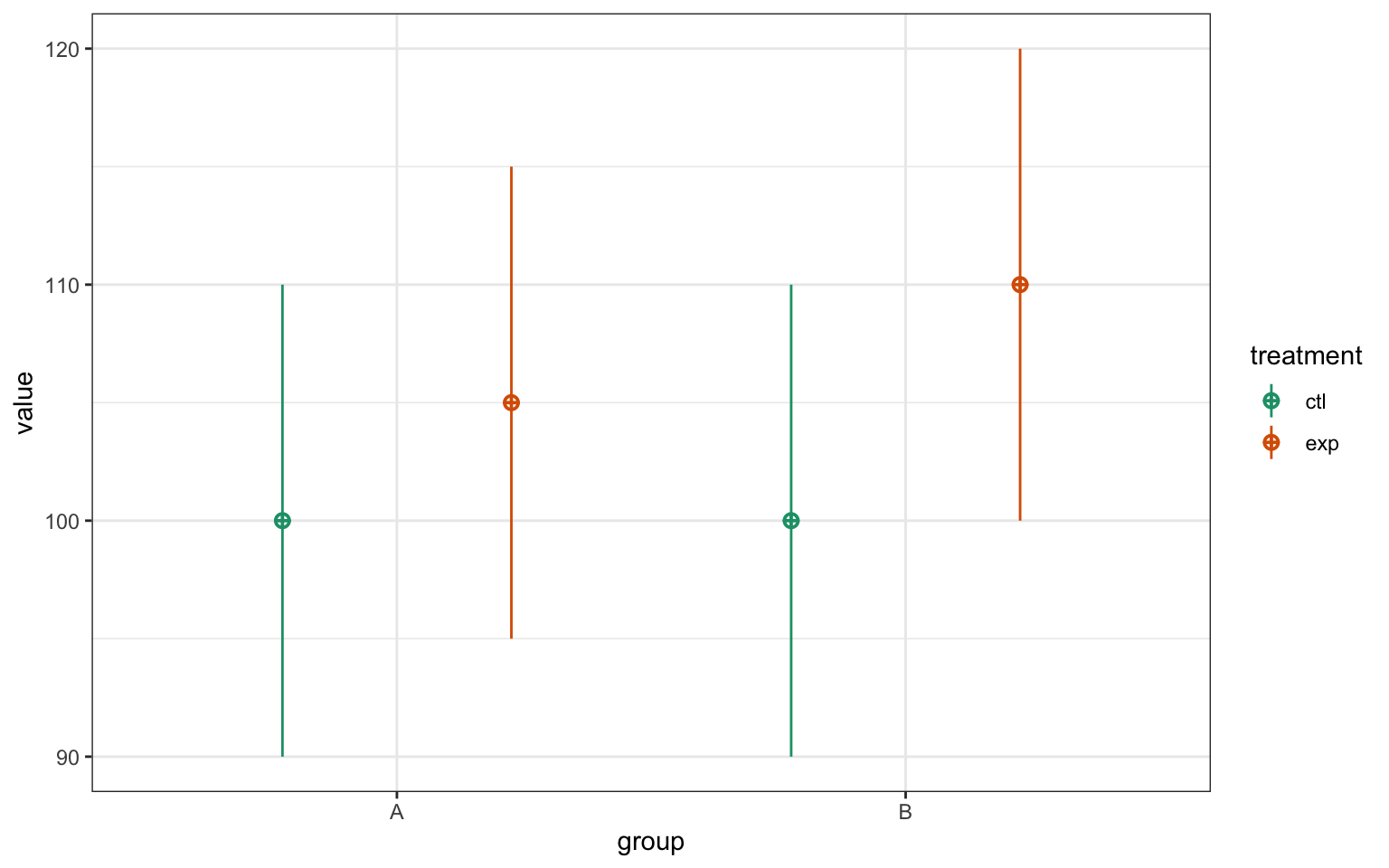
Figure 6.1: CAPTION THIS FIGURE!!
Then we model the data using a [linear model])g.html#general-linear-model).
# model using lm
model <- lm(y ~ treatment * group, data = simdat)
summary(model)
#>
#> Call:
#> lm(formula = y ~ treatment * group, data = simdat)
#>
#> Residuals:
#>     Min      1Q  Median      3Q     Max
#> -28.086  -7.198  -0.092   6.872  35.072
#>
#> Coefficients:
#>                     Estimate Std. Error t value Pr(>|t|)
#> (Intercept)           99.056      1.065  92.967  < 2e-16 ***
#> treatmentexp           5.357      1.507   3.555 0.000423 ***
#> groupB                 1.236      1.507   0.820 0.412703
#> treatmentexp:groupB    4.827      2.131   2.265 0.024036 *
#> ---
#> Signif. codes:  0 '***' 0.001 '**' 0.01 '*' 0.05 '.' 0.1 ' ' 1
#>
#> Residual standard error: 10.65 on 396 degrees of freedom
#> Multiple R-squared:  0.1503, Adjusted R-squared:  0.1439
#> F-statistic: 23.35 on 3 and 396 DF,  p-value: 6.17e-14
Use the emmeans package to get the estimated marginal means from this model. You can get the estimated means for each combination of treatment and group:
emmeans::emmeans(model, ~ treatment | group)
#> group = A:
#>  treatment emmean   SE  df lower.CL upper.CL
#>  ctl         99.1 1.07 396     97.0      101
#>  exp        104.4 1.07 396    102.3      107
#>
#> group = B:
#>  treatment emmean   SE  df lower.CL upper.CL
#>  ctl        100.3 1.07 396     98.2      102
#>  exp        110.5 1.07 396    108.4      113
#>
#> Confidence level used: 0.95
Or for the main effects separately (there will be a warning that the interaction may make this misleading).
emmeans::emmeans(model, ~ treatment)
#> NOTE: Results may be misleading due to involvement in interactions
#>  treatment emmean    SE  df lower.CL upper.CL
#>  ctl         99.7 0.753 396     98.2      101
#>  exp        107.4 0.753 396    106.0      109
#>
#> Results are averaged over the levels of: group
#> Confidence level used: 0.95
emmeans::emmeans(model, ~ group)
#> NOTE: Results may be misleading due to involvement in interactions
#>  group emmean    SE  df lower.CL upper.CL
#>  A        102 0.753 396      100      103
#>  B        105 0.753 396      104      107
#>
#> Results are averaged over the levels of: treatment
#> Confidence level used: 0.95
6.12 extension
The end part of a file name that tells you what type of file it is (e.g., .R or .Rmd).
Common file types and their extensions
| File type | extension |
|---|---|
| R script | .R |
| R Markdown | .Rmd |
| Comma-separated variable | .csv |
| SPSS data file | .sav |
| Plain text | .txt |
| Web file | .html |
| Word document | .doc, .docx |
Often extensions are forgotten when importing files (e.g., reading data files into R) or when exporting files (e.g., saving plots as pictures).
6.13 extract operator
A symbol used to get values from a container object, such as [, [[, or $
You can extract values from a vector by index or name using [ and [[.
my_vector <- c(A = "first", B = "second")
my_vector[1]   # by index, retains name
#>       A
#> "first"
my_vector[[1]] # by index, removes name
#> [1] "first"
my_vector["B"] # by name, retains name
#>        B
#> "second"
my_vector[["B"]] # by name, removes name
#> [1] "second"
You can extract values from a list by index or name using [ and [[ and by name using $.
my_list <- list(
  A = "First item",
  B = 2
)

my_list[1]     # by index, returns a (named) list
#> $A
#> [1] "First item"
my_list[[1]]   # by index, returns an (unnamed) vector
#> [1] "First item"
my_list["B"]   # by name, returns a (named) list
#> $B
#> [1] 2
my_list[["B"]] # by name, returns an (unnamed) vector
#> [1] 2
my_list$A      # by name, returns an (unnamed) vector
#> [1] "First item"