4 C
4.1 cache
Storing information for later retrieval, usually to save time.
In R Markdown documents, you can cache time-consuming code chunks, such as running a complex mixed effects model, by adding a chunk option cache = TRUE.
4.2 cache (web)
In a web browser, external files like CSS, JavaScript, and images are usually cached so that they don't have to be repeatedly downloaded.
When you are developing Shiny apps, you may find that your styles, scripts, or images don't update, even though you've changed the source files. This is usually because of the cache, and you can fix it by reloading the web browser, or restarting R and rerunning the Shiny app.
4.4 character
A data type representing strings of text.
Examples of character data are:
"I am a string of characters"
#> [1] "I am a string of characters"
paste("The answer is ", 6+6)
#> [1] "The answer is  12"
as.character(100)
#> [1] "100"
4.5 chunk
A section of code in an R Markdown file
In an Rmd file, you can include a chunk by surrounding the code as in the example below:
Also sometimes called a block.
4.6 CI
Confidence interval: A type of interval estimate used to summarise a given statistic or measurement where a proportion of intervals calculated from the sample(s) will contain the true value of the statistic.
4.7 class
A way to categorise objects
A class is similar to a data type, but object can have more than one class.
More...
# function class and closure type
class(mean)
#> [1] "standardGeneric"
#> attr(,"package")
#> [1] "methods"
typeof(mean)
#> [1] "closure"
Classes often control how an object is printed. For example, the result of t.test() is a list with class "htest", which is why printing the result gives you formatted output.
t <- t.test(rnorm(10), rnorm(10))
typeof(t)
#> [1] "list"
class(t)
#> [1] "htest"
t
#>
#>  Welch Two Sample t-test
#>
#> data:  rnorm(10) and rnorm(10)
#> t = -0.87885, df = 16.532, p-value = 0.3921
#> alternative hypothesis: true difference in means is not equal to 0
#> 95 percent confidence interval:
#>  -1.5093996  0.6230434
#> sample estimates:
#>   mean of x   mean of y
#> -0.07360206  0.36957606
If you unclass() an object, it no longer gets specical printing styles.
unclass(t)
#> $statistic
#>         t
#> -0.878845
#>
#> $parameter
#>       df
#> 16.53224
#>
#> $p.value
#> [1] 0.3920801
#>
#> $conf.int
#> [1] -1.5093996  0.6230434
#> attr(,"conf.level")
#> [1] 0.95
#>
#> $estimate
#>   mean of x   mean of y
#> -0.07360206  0.36957606
#>
#> $null.value
#> difference in means
#>                   0
#>
#> $stderr
#> [1] 0.5042733
#>
#> $alternative
#> [1] "two.sided"
#>
#> $method
#> [1] "Welch Two Sample t-test"
#>
#> $data.name
#> [1] "rnorm(10) and rnorm(10)"
4.8 coding scheme
How to represent categorical variables with numbers for use in models
- effect code
- sum code
- treatment code (dummy code)
Example of different coding schemes for the same data
Contrast coding in R by Marissa Barlaz
4.9 coercion
Changing the data type of values in a vector to a single compatible type.
If you try to combine values with different data types in a vector or matrix, they get coerced to a common type. Strings are most dominant which means, if you try to combine a string with another data type, the other data type will be coerced into a string. Doubles are dominant over integers and numeric values are dominant over logical values.
4.10 comment
Comments are text that R will not run as code. You can annotate .R files or chunks in R Markdown files with comments by prefacing each line of the comment with one or more hash symbols (#).
# I'm demonstrating comments in this chunk
# This comment will be added to the document outline ----
You can comment multiple lines at once by highlighting the code you would like to change into a comment and using the keyboard shortcut Ctrl + Shift + C (Windows) or Command + Shift + C (Mac). You can also change from comment to code (un-commenting) by using the same keyboard shortcut.
Comments get added to the document outline if you put four or more dashes, equal signs, or hashes at the end. This is a great way to keep track of more complicated scripts.
4.11 commit
The action of storing a new snapshot of a project's state in the git history.
4.12 compile
To create another resource, such as an app, from source code.
Compiling usually refers to taking human-readable code and converting it into code that is more efficient for a computer to run, but that a human can't read.
In the context of R Markdown files, knit, render and compile are sometimes used interchangeably.
4.13 computational reproducibility
The extent to which the findings of a study can be repeated with the same raw data but analyzed by different researchers or by the same researchers on a different occasion.
See also reproducibility.
4.14 concatenate
To combine strings or vectors.
When referring to strings, concatenate means to add strings together using the function paste (adds a space between strings) or paste0 (doesn't add anything between strings).
subject_name <- "Lisa"
paste("Hello,", subject_name)
#> [1] "Hello, Lisa"
When referring to other types of variables, concatenate can mean to create a vector with those variables, usually using the c function. For example, you could concatenate the numbers 1, 3, 6, and 10 like this: c(1, 3, 6, 10). You can concatenate two vectors as well:
v1 <- 1:5
v2 <- 11:15
c(v1, v2)
#> [1] 1 2 3 4 5 11 12 13 14 154.15 confidence interval
A type of interval estimate used to summarise a given statistic or measurement where a proportion of intervals calculated from the sample(s) will contain the true value of the statistic.
For example, 95% Confidence Intervals of the mean state that if you were to run the same study on 100 samples and calculate this interval for each iteration of the study, then 95 of the intervals calculated will contain the true mean of the population.
Most commonly cited Confidence Intervals are the 95% Confidence Interval and the 99% Confidence Interval. The 95% CI and 99% CI of the mean are calculated as follows:
- \(95\%\ CI = \mu ± 1.96 \times SD\)
- \(99\%\ CI = \mu ± 2.58 \times SD\)
For example, given \(\mu\) = 10 and \(SD\) = 1.25, the \(95\%\ CI = [7.55, 12.45]\)
There are a number of misconceptions about Confidence Intervals and it would be worth reading the following papers:
4.16 conflict
Having two packages loaded that have a function with the same name.
For example, when you load the tidyverse, you will see several warnings under the Conflicts heading.
── Conflicts ───── tidyverse_conflicts() ──
x dplyr::filter() masks stats::filter()
x lag()::filter() masks stats::lag()
This means that the stats package has functions called filter() and lag(), but the dplyr package (part of the tidyverse), also has functions with the same name.
Because you loaded dplyr after stats (which is loaded by default when you start R), the functions from dplyr mask the functions from stats, but you can still use the functions from stats, you just need to preface them with stats::.
More...
Sometime, the two functions do totally different things. There just aren't enough names to go around; this is why all packages aren't loaded by default. For example, stats::filter() applies linear filtering to a time series, while dplyr::filter() subsets a data frame.
stats::filter(1:10, rep(1, 3))
#> Time Series:
#> Start = 1
#> End = 10
#> Frequency = 1
#> [1] NA 6 9 12 15 18 21 24 27 NA| country | year | cases | population |
|---|---|---|---|
| Afghanistan | 1999 | 745 | 19987071 |
| Afghanistan | 2000 | 2666 | 20595360 |
In other cases, a package will name a function the same as a base R function on purpose, in order to do the same thing with more features. For example, base::setdiff() and dplyr::setdiff() both return rows from the first table that are not in the second table, but the base R version requires columns to be in the same order, while the dplyr version does not.
# define overlapping tables
t1 <- data.frame(a = 1:3, b = 1:3)
t2 <- data.frame(b = 2:4, a = 2:4)

# concludes all t1 rows are not in t2
base::setdiff(t1, t2)
#> $a
#> [1] 1 2 3
# concludes only 1 t1 row is not in t2
dplyr::setdiff(t1, t2)| a | b |
|---|---|
| 1 | 1 |
4.17 console
The pane in RStudio where you can type in commands and view output messages.
Commands typed into the console are not saved in a script, although they may be saved in the history.
4.18 container
A data structure that aggregates data, such as a vector, list, matrix, or data frame
# vector
c(1,2,3,4)
#> [1] 1 2 3 4
# list
list(1, "A", TRUE)
#> [[1]]
#> [1] 1
#>
#> [[2]]
#> [1] "A"
#>
#> [[3]]
#> [1] TRUE
# matrix
matrix(1:6, nrow = 2)
#>      [,1] [,2] [,3]
#> [1,]    1    3    5
#> [2,]    2    4    6
# data frame
data.frame(
  id = 1:5,
  name = c("Lisa", "Phil", "Helena", "Rachel", "Jack")
)| id | name |
|---|---|
| 1 | Lisa |
| 2 | Phil |
| 3 | Helena |
| 4 | Rachel |
| 5 | Jack |
A container may also refer to a virtual software environment that can be used to make sure that your code has the intended versions of all packages. Docker, Binder and Code Ocean are popular conatiner types.
4.19 continuous
Data that can take on any values between other existing values.
As opposed to discrete data, where fractional values don't make sense, continuous data can take fractional values (as far as the sensitivity of the measurement allows). So even if you are measuring height to the nearest whole centimeter, this is continuous data because it is possible and makes sense for intermediate values to exist.
4.20 correlation matrix
Parameters showing how a set of vectors are correlated.
This is set up as a matrix with 1.0 along the diagonal, meaning that every variable is perfectly correlated with itself.
data <- tibble(
  A = rnorm(100),
  B = rnorm(100), # uncorrelated with A
  C = rnorm(100) + A, # positively correlated with A
  D = rnorm(100) - A # negatively correlated with A
)

cor(data) # correlation matrix
#>               A             B           C           D
#> A  1.0000000000 -0.0009943199  0.66356312 -0.69155202
#> B -0.0009943199  1.0000000000 -0.03771143 -0.04160253
#> C  0.6635631226 -0.0377114274  1.00000000 -0.39843597
#> D -0.6915520161 -0.0416025327 -0.39843597  1.00000000
4.21 correlation
The relationship two vectors have to each other.
If you sample two sets of numbers independently, they will have a correlation close to 0 (on average). If one number perfectly predicts the other, the correlation is 1 if one gets bigger as the other gets bigger and -1 if one gets smaller as the other gets smaller.
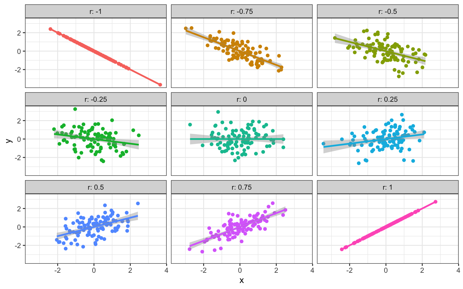
Figure 4.1: Different Correlations (n = 100)
4.22 covariance matrix
Parameters showing how a set of vectors vary and covary.
The covariance matrix is related to the correlation matrix, but also incorporates information about the standard deviations of all the variables.
More...
data <- faux::rnorm_multi(
  n = 100,
  mu = 0,
  sd = c(A = 1, B = 2, C = 3),
  r = 0.5,
  empirical = TRUE
)

cor(data) # correlation matrix
#>     A   B   C
#> A 1.0 0.5 0.5
#> B 0.5 1.0 0.5
#> C 0.5 0.5 1.0
cov(data) # covariance matrix
#>     A B   C
#> A 1.0 1 1.5
#> B 1.0 4 3.0
#> C 1.5 3 9.0
The matrix of the products of the standard deviations is called "sigma". If you multiply this by the correlation matrix, you get the covariance matrix.
4.23 covariance
The relationship two vectors have to each other.
A positive covariance means that as one vector increases the other does as well. A negative covariance means that as one vector increases the other decreases. A covariance of 0 means that the two vectors have to relation to each other.
Covariances can take on any numerical value which can make them difficult to interpret. Because of this covariances are often converted into correlations by incorporating information about each vectors' standard deviations.
4.24 covariate
Characteristics of the observations in a study that may affect the response variable.
Covariates can be independent variables of interest in your analysis, or confounding variables.
In the context of ANCOVAs, covariate specifically refers to continuous predictor variables.
4.25 CRAN
The Comprehensive R Archive Network: a network of ftp and web servers around the world that store identical, up-to-date, versions of code and documentation for R.
Packages that you download from CRAN have been checked to make sure they won't harm your computer. You can learn more about CRAN at https://cran.r-project.org/.
4.26 Cronbach's alpha
A measure used to assess the internal consistency of scale items
If a scale is a reliable measure of a concept, then the items of the scale should consistently measure that concept. A scale where all the items perfectly measure the same concept will have a Cronbach's alpha close to 1.0, basically meaning that all the items are nearly perfectly correlated. A scale where each item measures a totally different concept will have a Cronbach's alpha close to 0.0, meaning that each item is uncorrelated with the others.
Remember that internal reliability is not the same as external reliability. A scale can have a very high Cronbach's alpha, meaning it measures something well, but that thing may not be what you meant to measure.
More...
We can use the function psych::alpha() to calculate Cronbach's alpha.
# read in data from the 3 domains of disgust scale
disgust <- readr::read_csv("https://psyteachr.github.io/msc-data-skills/data/disgust.csv")

# select just the items that measure pathogen disgust
pathogen_alpha <- disgust %>%
  select(pathogen1:pathogen7) %>%
  psych::alpha()
You often just want to report the raw or standard alpha.
pathogen_alpha$total$raw_alpha
#> [1] 0.7379495
pathogen_alpha$total$std.alpha
#> [1] 0.744352
The item.stats section gives you some descriptive statistics about each item (see ?psych::alpha for more info).
pathogen_alpha$item.stats| n | raw.r | std.r | r.cor | r.drop | mean | sd | |
|---|---|---|---|---|---|---|---|
| pathogen1 | 19668 | 0.6035673 | 0.6268390 | 0.5298980 | 0.4530070 | 4.443156 | 1.457303 |
| pathogen2 | 19683 | 0.6371098 | 0.6288656 | 0.5372173 | 0.4610671 | 3.254026 | 1.745723 |
| pathogen3 | 19687 | 0.6489288 | 0.6601790 | 0.5845474 | 0.4917248 | 3.171941 | 1.616815 |
| pathogen4 | 19683 | 0.6217909 | 0.6169971 | 0.5159811 | 0.4397615 | 3.657573 | 1.755883 |
| pathogen5 | 19678 | 0.6384423 | 0.6658879 | 0.5921973 | 0.4997309 | 4.282397 | 1.435962 |
| pathogen6 | 19655 | 0.6120328 | 0.5924165 | 0.4787382 | 0.4119616 | 3.808751 | 1.878335 |
| pathogen7 | 19692 | 0.6331624 | 0.6062995 | 0.5021699 | 0.4326954 | 3.493500 | 1.930726 |
You can look at the alpha.drop section to see what the alpha would be if you dropped an item. If we add an item from the moral disgust scale, you can see that the alpha increases if you drop it.
mixed_alpha <- disgust %>%
  select(pathogen1:pathogen7, moral1) %>%
  psych::alpha()

select(mixed_alpha$alpha.drop, raw_alpha, std.alpha)| raw_alpha | std.alpha | |
|---|---|---|
| pathogen1 | 0.6776276 | 0.6874901 |
| pathogen2 | 0.6770689 | 0.6905960 |
| pathogen3 | 0.6693926 | 0.6801944 |
| pathogen4 | 0.6787991 | 0.6913464 |
| pathogen5 | 0.6704759 | 0.6779193 |
| pathogen6 | 0.6860804 | 0.6982704 |
| pathogen7 | 0.6823258 | 0.6952413 |
| moral1 | 0.7379495 | 0.7443520 |
4.27 CSS
Cascading Style Sheet: A system for controlling the visual presentation of HTML in web pages.
R Markdown scripts are often knit to HTML. Therefore, you can also include HTML (a way to semantically tag information) and CSS in your scripts.
Here is an example of some simple CSS (in the style tag) and HTML.
<style>
  h3 { color: red; }
  .ferret { width: 200px; height: 150px; }
</style>

<h3>Red Title</h3>

<img src="images/darwin.jpg"
     title="The cutest ferret"
     class="ferret">
Resources