20 S
20.1 sample
A subset of the population that you wish to make an inference about through your test.
The sample is a smaller group obtained from your population, but it is key that the sample is representative of the population.
In most instances, it is realistically impossible to test all members of a population. A sample is derived from the population of interest to represent that population. The sample should have the same demographic characteristics as the population, for example. If your sample is not representative of the population, then any conclusions derived from your test may be invalid.
If the population is small enough to feasibly test in full, e.g. all students in a final year Psychology class, then your sample and the population are the same.
More...
In R, sample() is a function which can be used to pull an arbitrary number of elements from a vector. For instance, you can use sample to randomly draw five numbers (with or without replacement) from a vector containing the numbers 1 to 10:
set.seed(4491) # set seed for reprodicibilty
# create a vector containing the numbers 1 to 10
v <- 1:10
v
#>  [1]  1  2  3  4  5  6  7  8  9 10

# sample 5 numbers from v without replacement
sample(v, 5)
#> [1]  2  7  9 10  5
# sample 5 numbers from v with replacement
sample(v, 5, replace = TRUE)
#> [1]  1  8  6 10  1
For an interesting paper on populations, samples and generalisability, see:
- Simons, D. J., Shoda, Y., & Lindsay, D. S. (2017). Constraints on Generality (COG): A Proposed Addition to All Empirical Papers. Perspectives on Psychological Science, 12(6), 1123–1128. doi: 10.1177/1745691617708630
20.2 scientific notation
A number format for working with very large or small numbers.
Numbers are most commonly written in decimal notation, like 3.145 or 365. However, when numbers are very large or small, it's difficult to read or write them correctly.
More...
For example, Avogadro's constant, the number of particles contained in one mole of any substance, is equal to 602,252,000,000,000,000,000,000. The commas make it a little easier to parse when reading, but you can't use those in coding. The scientific notation is \(6.02x10^{23}\), which means the you multiply 6.02 times the number that is 1 with 23 zeros after it (or move the decimal place in 6.02 23 places to the right). In R, this notation looks like 6.02e23.
Negative numbers move the decimal place to the left. For example, Wyler's constant in physics is 1.05e-109, or a decimal place followed by 108 zeros before you get to the first non-zero digit.
    0.0001 == 1e-4
    0.001  == 1e-3
    0.01   == 1e-2
    0.1    == 1e-1
    1      == 1e0
   10      == 1e1
  100      == 1e2
 1000      == 1e3
10000      == 1e4
You can format numbers with scientific notation in R using the function formatC(). This turns them into text that you can use in inline code, but you can't use as a number anymore.
x <- c(123456789, 0.06789, 0.000000012)
formatC(x, format = "e", digits = 2)
#> [1] "1.23e+08" "6.79e-02" "1.20e-08"
Model output can often contain numbers in scientific notation. To change the threshold at which large or small numbers display with scientific notation, set the scipen option at the top of a script. A value of 0 means that R will use scientific notation whenever that representation takes less space than the decimal representation. Larger values make decimal notation more likely and smaller values make scientific notation more likely.
test <- list(1000000,
              100000,
               10000,
                1000,
                 100,
                  10,
                   1,
                   0.1,
                   0.01,
                   0.001,
                   0.0001,
                   0.00001,
                   0.000001)
options(scipen = 1)
str(test)
#> List of 13
#>  $ : num 1e+06
#>  $ : num 100000
#>  $ : num 10000
#>  $ : num 1000
#>  $ : num 100
#>  $ : num 10
#>  $ : num 1
#>  $ : num 0.1
#>  $ : num 0.01
#>  $ : num 0.001
#>  $ : num 0.0001
#>  $ : num 1e-05
#> $ : num 1e-0620.3 scope
The environment where an object is available
The main thing you need to know about scope involves writing your own functions. Objects created outside of a function (e.g., in the console or in a script are global variables that are accessible throughout your R session. Objects created inside a function are local variables that are only available inside the function and not outside.
y <- 5 # this y is global

x <- function() {
  y <- 10 # this y is local
  return(y)
}

x() # returns the local value of y
#> [1] 10
y # returns the global value of y
#> [1] 5
If you have arguments to a function, they are local variables inside the function and their values will overwrite any global variables with the same name.
y <- 5 # this y is global

x <- function(y) {
  y <- y + 1 # this uses the local value of y
  return(y)
}

x(10) # returns 10 + 1
#> [1] 11
y     # y is still 5
#> [1] 520.6 semi_join
A filtering join that returns all rows from the left table where there are matching values in the right table, keeping just columns from the left table.
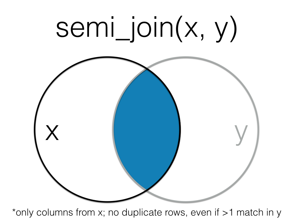
Figure 20.1: Semi Join
This is useful when you have a table of data that contains IDs of data that passes your exclusion criteria.
all_data <- tibble(
  id = 1:5,
  x = LETTERS[1:5]
)

to_keep <- tibble(
  id = 2:4
)

data <- semi_join(all_data, to_keep, by = "id")| id | x |
|---|---|
| 2 | B |
| 3 | C |
| 4 | D |
See joins for other types of joins and further resources.
20.7 server
This is the part of a Shiny app that works with logic.
The server is a function that processes the user's input in the UI, and allows the app to render appropriate output. See this shiny basics article for more.
20.8 SESOI
Smallest Effect Size of Interest: the smallest effect that is theoretically or practically meaningful
See Equivalence Testing for Psychological Research: A Tutorial for a tutorial on methods for choosing an SESOI.
Lakens, D. (2017a). Equivalence tests: A practical primer for t tests, correlations, and meta-analyses. Social Psychological & Personality Science, 8, 355–362. doi:10.1177/1948550617697177
20.9 set operations
Functions that compare two tables and return rows that match (intersect), are in either table (union), or are in one table but not the other (setdiff).
The examples below use two small datasets. a has ids 1 to 5, and b has ids 3 to 7.
intersect() returns all rows in two tables that match exactly. The columns don't have to be in the same order.
dplyr::intersect(a, b)| id |
|---|
| 3 |
| 4 |
| 5 |
union() returns all the rows from both tables, removing duplicate rows.
dplyr::union(a, b)| id |
|---|
| 1 |
| 2 |
| 3 |
| 4 |
| 5 |
| 6 |
| 7 |
setdiff returns rows that are in the first table, but not in the second table.
dplyr::setdiff(a, b)| id |
|---|
| 1 |
| 2 |
If you've forgotten to load dplyr or the tidyverse, base R also has these functions. You will either get an error message or unexpected output if you try to use them with data tables.
20.11 shinydashboard
A package for R that builds on Shiny for more flexible and visually appealing UIs.
Shiny Dashboard or shinydashboard can be installed with install.packages("shinydashboard"), and can be loaded with library(shinydashboard). The shinydashboard documentation is a great introduction to this package.
20.14 single brackets
A pair of square brackets used to select a subset from a container like a list, data frame, or matrix (e.g., data[1, ]).
secret_code <- c(16, 19, 25, 20, 5, 1, 3, 8, 18)

LETTERS[secret_code]
#> [1] "P" "S" "Y" "T" "E" "A" "C" "H" "R"
See brackets for an explanation of the difference between single and double brackets.
20.15 slope
A quantity that captures how much change in one variable is associated with a unit increase in another variable.
If you have a slope of 3, that means that a unit increase in the \(X\) variable is associated with a 3 unit change in the \(Y\) variable. If you have a slope of -1/2, then a unit increase in the \(X\) variable is associated with a decrease of 1/2 in the \(Y\) variable.
20.16 standard deviation
A descriptive statistic that measures how spread out data are relative to the mean.
If the data points are further from the mean, there is a higher standard deviation. Standard deviation is calculated as the square root of the variance.
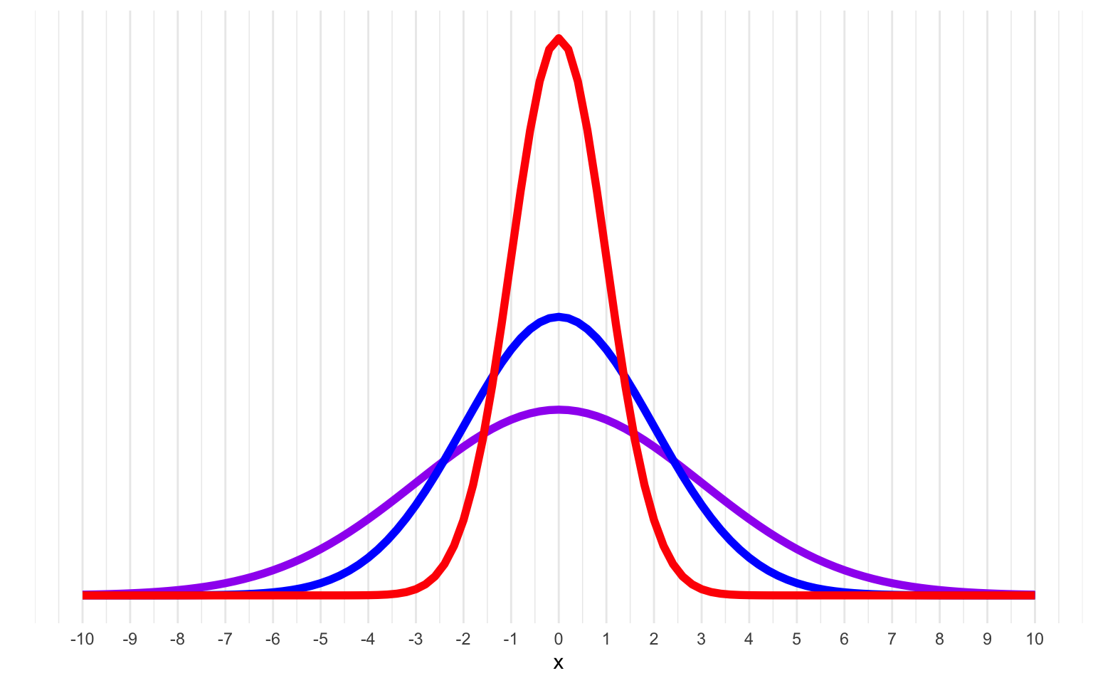
Figure 20.2: Normal distributions with means of 0 and SDs of 1 (red), 2 (blue) and 3 (purple).
20.17 standardize
The process of putting vectors on the same scale. In statistics, this often means that a vector has a mean of 0 and a standard deviation of 1.
You can standardize a vector by subtracting the vector mean from each value
and then dividing each each difference by the vector standard deviation, or by using the scale() function.
More...
Standardize a vector manually:
# create a vector containing the numbers 1 to 10
v <- 1:10

# calculate mean and SD
v_mean <- mean(v)
v_sd <- sd(v)

# standardize
standardized_v <- (v - v_mean) / v_sd

data.frame(
  original = v,
  standardized = standardized_v
)| original | standardized |
|---|---|
| 1 | -1.4863011 |
| 2 | -1.1560120 |
| 3 | -0.8257228 |
| 4 | -0.4954337 |
| 5 | -0.1651446 |
| 6 | 0.1651446 |
| 7 | 0.4954337 |
| 8 | 0.8257228 |
| 9 | 1.1560120 |
| 10 | 1.4863011 |
Now the mean and standard deviation of the new vector will be 0 and 1
You can also use the scale() function in R to automate the standardization process.
The result of the scale() function is a 2-dimensional matrix, so you usually need to extract the vector of values like this:
scaled_v[, 1]
#>  [1] -1.4863011 -1.1560120 -0.8257228 -0.4954337 -0.1651446  0.1651446
#>  [7]  0.4954337  0.8257228  1.1560120  1.4863011
20.18 static
Something that does not change in response to user actions
For example, in a shiny app, the following code creates static and dynamic elements.
static <- shiny::p("This text cannot change")
dynamic <- shiny::textOutput("This text can change")
20.19 string
A piece of text inside of quotes.
For example, "I sense the rains down in Africa" is a string. Numbers inside of quotes can be a string; "19" is a string, while 19 is not.
20.20 sum code
A coding scheme for categorical variables that compares the mean for each level to the overall mean.