3 B

3.1 base R

The set of R functions that come with a basic installation of R, before you add external packages.

Contrast with tidyverse.

完成基本安裝，啟動R就自動載入的函式庫。自行安裝的外部套件，例如tidyverse，需要手動載入。

3.2 beta distribution

A family of distributions of data that are characterised by two parameters: α and β

Wikipedia actually has really good definitions and examples.

3.3 beta

The false negative rate we accept for a statistical test.

Beta is equal to 1 minus power, so if a test has power of 0.8 for a specific effect size and alpha, then beta = 0.2.

Beta can also refer to a parameter of the beta distribution

3.4 between subjects

Not varying within unit of observation, such that each has only one value

For example, imagine an experiment where you test half of subjects in a dark room and the other half in a light. This experiment has one factor, room darkness, which is between subjects because each subject only experiences one level of room darkness, not both. This experiment may also be described as "between subjects".

Contrast with within subjects.

3.5 bind_cols

A binding join that joins one table to another by adding their columns together

bind_cols takes two tables with the same number of rows and adds the columns from the second table to the first.

a <- tibble(
  id = 1:3,
  x = LETTERS[1:3]
)

b <- tibble(
  y = c(T, T, F)
)

data <- dplyr::bind_cols(a, b)

id	x	y
1	A	TRUE
2	B	TRUE
3	C	FALSE

If any column has the same name in both tables, you will see a warning that the columns have been given new names.

a <- tibble(
  id = 1:3,
  x = LETTERS[1:3]
)

b <- tibble(
  x = c(T, T, F)
)

data <- dplyr::bind_cols(a, b)
#> New names:
#> • `x` -> `x...2`
#> • `x` -> `x...3`

id	x...2	x...3
1	A	TRUE
2	B	TRUE
3	C	FALSE

See joins for other types of joins and further resources.

3.6 bind_rows

A binding join that joins one table to another by adding their rows together

bind_rows takes two tables, finds all columns with the same name, and appends the second one to the first. If a column doesn't have a match in the other table, that columns' values are set to NA.

a <- tibble(
  id = 1:3,
  x = LETTERS[1:3],
  y = c(T, T, F)
)

b <- tibble(
  x = LETTERS[4:6],
  id = 4:6
)

data <- dplyr::bind_rows(a, b)

id	x	y
1	A	TRUE
2	B	TRUE
3	C	FALSE
4	D	NA
5	E	NA
6	F	NA

See joins for other types of joins and further resources.

3.7 binding joins

Joins that bind one table to another by adding their rows or columns together.

• bind_rows
• bind_cols

3.8 binomial distribution

The distribution of data where each observation can have one of two outcomes, like success/failure, yes/no or head/tails.

# flip 10 coins 10000 times
x <- rbinom(10000, 10, prob = 0.5)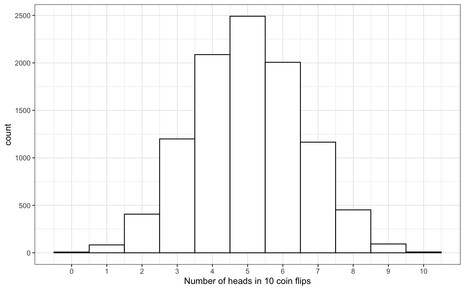

Figure 3.1: Binomial Distribution

3.9 bivariate normal

Two normally distributed vectors that have a specified correlation with each other.

You can use the {faux} package to quickly create variables from a bivariate normal distribution with a specified correlation.

data <- faux::rnorm_multi(
  n = 10000, vars = 2, 
  mu = 0, sd = 1, r = 0.5,
  varnames = c("x", "y")
)

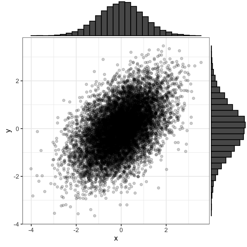
Figure 3.2: A bivariate normal distribution where both variables have mu = 0 and SD = 1, with r = 0.5

3.10 block

A section of code in an R Markdown file

See chunk.

3.11 boolean expression

An expression that evaluates to TRUE or FALSE.

Boolean expressions usually use a relational operator, such as == or > to compare two values.

More...

# ==    Equal to    
1 == 1
#> [1] TRUE
1 == 2
#> [1] FALSE

# !=    Not equal to    
1 != 2
#> [1] TRUE
1 != 1
#> [1] FALSE

# >     Greater than
2 > 1
#> [1] TRUE
1 > 2
#> [1] FALSE

# >=    Greater than or equal to
2 >= 1
#> [1] TRUE
1 >= 2
#> [1] FALSE

# <     Less than
1 < 2
#> [1] TRUE
2 < 1
#> [1] FALSE

# <=    Less than or equal to
1 <= 2
#> [1] TRUE
2 <= 1
#> [1] FALSE

# %in%  Match operator  
"A" %in% LETTERS
#> [1] TRUE
"1" %in% LETTERS
#> [1] FALSE

3.12 boolean

A data type representing TRUE or FALSE values.

Typically called logical in R.

3.13 bootstrap

Resampling with replacement.

In statistics, bootstrapping is used to resample with replacement from an original small sample. This allows us to calculate confidence intervals for any estimate.

• A Practical Guide to the Bootstrap in R
• Bootstrapping by Quick-R

3.14 brackets

Square brackets used to subset a container like a vector, list, data frame, or matrix (e.g., mtcars[[1]] or mtcars[1:2]).

When you use single brackets to subset a container, you get back a container with the items you selected. This contrasts with double brackets, which only return a single item in the container.

More...

You can use single brackets to select one or more items from a vector.

secret_code <- c(16, 19, 25, 20, 5, 1, 3, 8, 18)

LETTERS[secret_code]
#> [1] "P" "S" "Y" "T" "E" "A" "C" "H" "R"

If you use double brackets, you can only select a single item from the vector. If you try to select more than one, you will get the following error messge.

LETTERS[[secret_code]]
#> Error in LETTERS[[secret_code]]: attempt to select more than one element in vectorIndex

You can select items by index or name. mylist[c("a", "c")] returns a list containing the first and third items.

mylist <- list(
  a = 10,
  b = 20,
  c = 30
)

mylist[c("a", "c")]
#> $a
#> [1] 10
#> 
#> $c
#> [1] 30

Single brackets return the same type of container as the object being subset, so mylist[1] returns a list containing just the first item.

mylist[1]
#> $a
#> [1] 10

Double brackets return the same type of object as the single item being selected, so mylist[[1]] returns a vector that is the same as the first item in mylist.

mylist[[1]]
#> [1] 10

Single brackets let you select rows and columns of a data frame or tibble, if you separate them by a comma.

data <- data.frame(
  id = 1:3,
  letter = c("a", "b", "c"),
  vowel = c(TRUE, FALSE, FALSE)
)

# rows 1:2 and columns 3:4
data[1:2, 2:3]

letter	vowel
a	TRUE
b	FALSE

If you omit the rows or columns, you select them all.

data[1, ] # row 1, all columns

id	letter	vowel
1	a	TRUE

data[, 1:2] # all rows, columns 1:2

id	letter
1	a
2	b
3	c

If you only select one column of a data frame with single brackets, you will get a vector back instead of a data frame. You can change this behaviour by using drop = FALSE.

data[, 1] # returns a vector
#> [1] 1 2 3

data[, 1, drop = FALSE] # returns a data frame

id
1
2
3

Tibbles always returns a tibble.

as_tibble(data)[, 1] # returns a tibble

id
1
2
3

Double brackets can be used with a single index or name to select a column as a vector.

data[["vowel"]]
#> [1]  TRUE FALSE FALSE

Or with row and column values to select a single cell.

data[[1, "vowel"]]
#> [1] TRUE

You can't use double brackets to select a single row of a data table.

data[[1, ]]
#> Error in `[[.data.frame`(data, 1, ): argument "..2" is missing, with no default

More complex containers like 3-dimensional arrays can have more than 2 values in the brackets, but work on the same principles.

myarray <- array(1:8, dim = c(2, 2, 2))
myarray[2, 2, 2]
#> [1] 8