7 F
7.1 factor
A data type where a specific set of values are stored with labels; An explanatory variable manipulated by the experimenter
7.2 factor (data type)
A data type where a specific set of values are stored with labels
In tables, you can store strings as characters or factors.
If you print a character vector, it will have quotes around each values, while a factor vector will show the Levels after.
data$chr
#> [1] "A" "B" "C"

data$fctr
#> [1] A B C
#> Levels: A B C
In a tibble, these types will have "<chr>" or "<fctr>" under the column header.
data| chr | fctr |
|---|---|
| A | A |
| B | B |
| C | C |
You can convert between characters and factors like this:
as.character(data$fctr)
#> [1] "A" "B" "C"

# set the levels to the order you want
factor(data$chr, levels = c("C", "B", "A"))
#> [1] A B C
#> Levels: C B A
Resources
- Factors in R for Data Science
7.3 factor (experimental)
An explanatory variable manipulated by the experimenter
For example, imagine an experiment where you test half of subjects in a dark room with easy, medium, and hard tasks, and the other half in a light room with easy and hard tasks. This experiment has two factors: room darkness and task difficulty. The factor of room darkness is between subjects and has two levels: dark and light. The factor of task difficulty is within subjects has three levels: easy, medium, and hard.
7.4 factorial
factorial): Experimental designs where all possible combinations of independent variables are considered; factorial): The mathematical operation where an integer is multiplied by every integer between 1 and itself
7.5 factorial (stats)
Experimental designs where all possible combinations of independent variables are considered.
For example, the following design has two factors: time and treatment, and all 4 combinations are represented in the data.
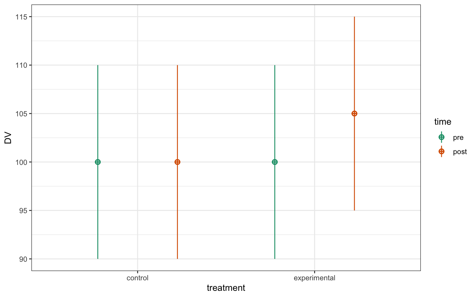
Figure 7.1: 2xw factorial data.
7.6 factorial (math)
The mathematical operation where an integer is multiplied by every integer between 1 and itself.
This operation is represented by an exclamation point in mathematical notation (e.g., 5!) and uses the factorial() function in R.
# 5 factorial
factorial(5)
#> [1] 120
5 * 4 * 3 * 2 * 1
#> [1] 120
7.7 false negative
When a test concludes there is no effect when there really is an effect
Also called a type II error, but we prefer the more descriptive "false negative".
See also true positive, true negative, false positive/type I error, and beta.
7.8 false positive
When a test concludes there is an effect when there really is no effect
Also called a type I error, but we prefer the more descriptive "false positive".
See also true positive, true negative, false negative/type II error, and alpha (stats).
7.9 filtering joins
Joins that act like the dplyr::filter() function in that they remove rows from the data in one table based on the values in another table.
The result of a filtering join will only contain rows from the left table and have the same number or fewer rows than the left table.
7.10 fitted value
The value of the response variable predicted by the model given certain values for any predictor variables.
If you have a model
\[Y_i = \beta_0 + \beta_1 X_i + e_i\]
then the fitted value for observation \(i\) equals \(\beta_0 + \beta_1 X_i\); that is, the model's prediction for a residual (\(e_i\)) of zero.
7.11 fixed effect
An effect assumed to be identical over all sampling units.
In the standard regression model
\[Y_i = \beta_0 + \beta_1 X_i + e_i\]
the parameters \(\beta_0\) (the intercept) and \(\beta_1\) (the slope) are assumed to be constant across all sampling units (e.g. subjects). These are contrasted with random effects, which are effects that differ across the units.
In a mixed effects model, you can get a table of just the fixed effects with the code below:
model <- afex::lmer(
  rating ~ rater_age * face_age + # fixed effects
  (1 | rater_id) + (1 | face_id), # random effects
  data = faux::fr4
)

broom.mixed::tidy(model, effects = "fixed")| effect | term | estimate | std.error | statistic | df | p.value |
|---|---|---|---|---|---|---|
| fixed | (Intercept) | 3.8109924 | 0.8815183 | 4.3232142 | 92.64738 | 0.0000387 |
| fixed | rater_age | 0.0041496 | 0.0251227 | 0.1651744 | 71.11697 | 0.8692753 |
| fixed | face_age | -0.0353353 | 0.0252691 | -1.3983587 | 92.18524 | 0.1653604 |
| fixed | rater_age:face_age | -0.0003824 | 0.0006174 | -0.6194014 | 712.00000 | 0.5358501 |
7.12 fixed factor
A factor whose levels are assumed to represent all the levels of interest in a population; its levels would remain fixed across replications of the study.
For example, if you were studying the nations making up the United Kingdom, you would have a factor with the levels England, Northern Ireland, Scotland, and Wales. If you would replicate a study, you would include these exact same levels. These four levels represent all the nations comprising the union, and there usually would be no interest in generalizing beyond the data to other (hypothetical) nations.
Fixed factors are usually contrasted with random factors, whose levels usually are assumed to be the result of (quasi-)random sampling.
7.13 formula
A symbolic expression that defines a model.
It takes a format like this:
y ~ 1 + x + z*w - z:w
The elements of the formula are:
-
~: on the left hand side, there is the outcome (y), on the right hand, the predictors. -
1: refers to the intercept that does not have to be written out as it is added by default. If you want to remove the intercept, you have to use 0 instead of 1. -
+: you can add predictors using the + sign. -
*: means to take two (or more) predictors, and use their main effect AND also their interaction.z*wtranslates intoz + w + z:w. -
:: refers to an interaction, without the main effects of the predictors. -
-: removes a predictor. For e.g.z*w - z:wtranslates into:z + w
In linear mixed effects model the formula also contains random effects. For example consider the following models:
y ~ x + (1|group)y ~ x + (x|group)y ~ x + (1|group/cluster)
-
(): defines the random effects. Can be more than one random effect. -
(1|group): adds a random intercept by group. -
(x|group): adds a random intercept and slope by group. -
(1|group/cluster): adds a random intercept by group nested in clusters. You can add more levels.
More info about adding random terms.
7.14 full_join
A mutating join that lets you join up rows in two tables while keeping all of the information from both tables
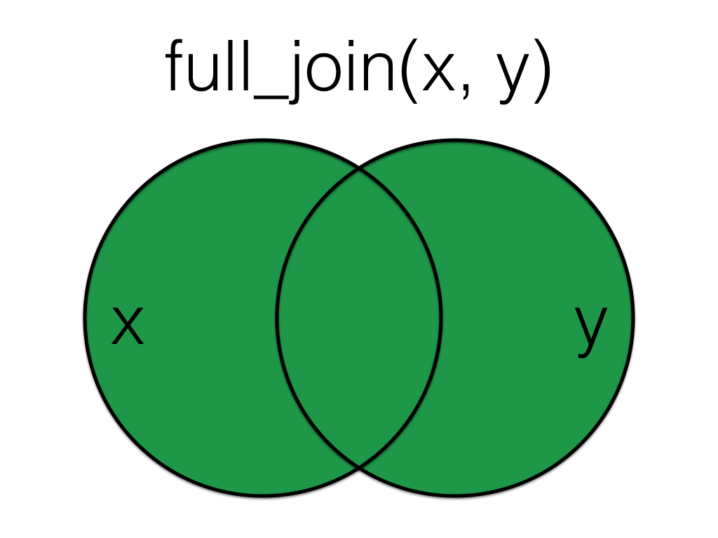
Figure 7.2: Full Join
More...
| Table X | Table Y | ||||||||||||||||||||||||
|---|---|---|---|---|---|---|---|---|---|---|---|---|---|---|---|---|---|---|---|---|---|---|---|---|---|
|
|
If there is no matching data in the other table for a row, the values are set to NA.
# X columns come first
data <- full_join(X, Y, by = "id")| id | x | y |
|---|---|---|
| 1 | A | NA |
| 2 | B | V |
| 3 | C | W |
| 4 | D | X |
| 5 | E | Y |
| 6 | NA | Z |
Order is not important for full joins, but does change the order of columns in the resulting table.
# Y columns come first
data <- full_join(Y, X, by = "id")| id | y | x |
|---|---|---|
| 2 | V | B |
| 3 | W | C |
| 4 | X | D |
| 5 | Y | E |
| 6 | Z | NA |
| 1 | NA | A |
See joins for other types of joins and further resources.
7.15 function
A named section of code that can be reused.
For example, sd is a function that returns the standard deviation of the vector of numbers that you provide as the input argument. Functions are set up like this: function_name(argument1 = a1, argument2 = a2). The arguments in parentheses can be named (like, x = c(1,3,5,8)) or you can skip the names if you put them in the exact same order that they're defined in the function. You can check this by typing ?sd (or whatever function name you're looking up) into the console and the Help pane will show you the default order under Usage.
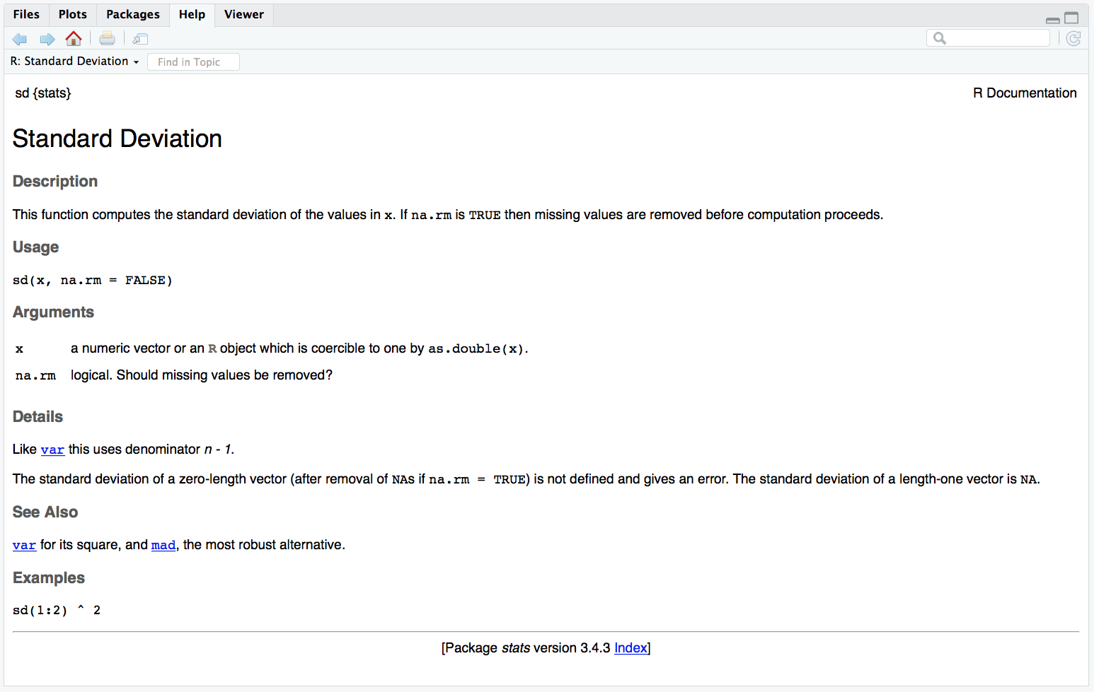
Figure 7.3: Function help