4  Data Summaries

Intended Learning Outcomes

• Be able to structure data for scripting
• Import data from CSV and Excel files
• Be able to summarise data by groups
• Be able to produce well-formatted tables
• Use pipes to chain together functions

Functions used

• built-in (you can always use these without loading any packages)
  • base:: c(), dput(), library(), max(), mean(), min(), sum()
  • stats:: quantile()
  • utils:: head()
• tidyverse (you can use all these with library(tidyverse))
  • readr:: cols(), col_factor(), col_skip(), read_csv(), spec()
  • dplyr:: arrange(), count(), desc(), filter(), glimpse(), group_by(), median(), mutate(), n(), summarise(), ungroup()
• other (you need to load each package to use these)
  • janitor:: clean_names()

Setup

TipActivity

1. Open your ADS-2026 project
2. Create a new quarto file called 04-data.qmd
3. Update the YAML header
4. Replace the setup chunk with the one below:

```{r}
#| label: setup
#| include: false

# packages needed for this chapter
library(tidyverse)     # loads readr for importing data
                       #   and tibble for creating tables
library(readxl)        # importing excel files
library(jsonlite)      # importing JSON files
library(rio)           # importing and exporting many types of files
library(skimr)         # summarising datasets
library(janitor)       # clean up data
```

You may also wish to download the Data import cheatsheet.

4.1 Import Data

The data we’ll be working with is on method of delivery for singleton births from Public Health Scotland. You can see the most recent version at Method of Delivery, but we’ll be working from a saved version. The data are in a CSV file, so we can read this with the function read_csv() , and assign it to a new object that we’ll call births. You can learn more about importing data from other file types in ?sec-data.

TipActivity

1. Download 12.1_delivery.csv), save it in your data folder, and then in a new code chunk, load in the data.

births <- read_csv("data/12.1_delivery.csv")

Rows: 97077 Columns: 9
── Column specification ────────────────────────────────────────────────────────
Delimiter: ","
chr (7): FinancialYear, CA, SIMDQuintileQF, SIMDVersion, AgeGroup, Delivery,...
dbl (2): SIMDQuintile, Livebirths

ℹ Use `spec()` to retrieve the full column specification for this data.
ℹ Specify the column types or set `show_col_types = FALSE` to quiet this message.

When you load data with read_csv(), you get a quick summary that you should always check to see if the data were loaded correctly. One common problem is that data load with the the wrong type (see Appendix D), usually because a numeric column contains some unexpected text values. So the first thing to check is that each column has the expected data type. The abbreviation “chr” means this is a character column, which can contain any text. The abbreviation “dbl” is a double, which is a number that can have decimal places.

There are too many columns to show all of them in the summary, so it tells you to use the spec() function to check all the columns.

spec(births)

cols(
  FinancialYear = col_character(),
  CA = col_character(),
  SIMDQuintile = col_double(),
  SIMDQuintileQF = col_character(),
  SIMDVersion = col_character(),
  AgeGroup = col_character(),
  Delivery = col_character(),
  Induced = col_character(),
  Livebirths = col_double()
)

This gives you the info formatted inside the cols() function to make it easy for you to copy and edit this if any of the columns imported incorrectly.

You can also use the glimpse() function to check the type of each column, and see a few examples of the cell values.

glimpse(births)

Rows: 97,077
Columns: 9
$ FinancialYear  <chr> "1997/98", "1997/98", "1997/98", "1997/98", "1997/98", …
$ CA             <chr> "RA2704", "RA2704", "RA2704", "RA2704", "RA2704", "RA27…
$ SIMDQuintile   <dbl> NA, NA, NA, NA, NA, NA, NA, NA, NA, NA, NA, NA, NA, NA,…
$ SIMDQuintileQF <chr> ":", ":", ":", ":", ":", ":", ":", ":", ":", ":", ":", …
$ SIMDVersion    <chr> "SIMD2004", "SIMD2004", "SIMD2004", "SIMD2004", "SIMD20…
$ AgeGroup       <chr> "25-34", "25-34", "25-34", "25-34", "25-34", "25-34", "…
$ Delivery       <chr> "Caesarean - Elective", "Caesarean - Emergency", "Caesa…
$ Induced        <chr> "Not Induced", "Induced", "Not Induced", "Induced", "No…
$ Livebirths     <dbl> 9, 5, 8, 1, 6, 21, 60, 4, 4, 3, 1, 1, 1, 14, 2, 6, 1, 7…

TipActivity

1. Run spec() on the dataset.
2. Run glimpse() on the dataset.

The column SIMDQuintileQF looks a little odd. We can quickly check what all the values are in a data table with the count() function:

count(births, SIMDQuintileQF)

SIMDQuintileQF	n
:	1137
NA	95940

It looks like this column doesn’t contain any useful info, so we can just ignore it, or skip it. We could do this later on by dropping the column using select() but it is also possible to amend the call to read_csv() so that it never gets loaded in the first place.

To do this at the point of loading in the data, we:

1. Create an object (birth_cols) that contains our column specification using the col_types argument and two helper functions, cols() and col_skip().
2. Pass birth_cols to the col_types argument of read_csv() which uses this info to amend the file that is loaded in.

TipActivity

1. Amend the code so that the column we do not need is skipped on loading.

# edit the output of spec(births)
birth_cols <- cols(
  SIMDQuintileQF = col_skip()
)

births <- read_csv("data/12.1_delivery.csv", col_types = birth_cols)

There’s also additional edits you can make to the initial file, for example, you can set the order of levels for categorical data when you first import it. This can be useful when you want to create plots as R will automatically order factors alphabetically but this might not be the most useful way to present your data. A very common option is to order your factor by importance or frequency of the groups.

To check which groups our data has, we can use the count() function to check the level labels for AgeGroup, Delivery and Induced; and set sort = TRUE to sort by frequency.

count(births, AgeGroup)

AgeGroup	n
25-34	37557
35 and over	29592
Under 25	29918
Unknown	10

count(births, Delivery, sort = TRUE)

Delivery	n
Spontaneous	25607
Caesarean - Emergency	22526
Forceps	19041
Vacuum	14573
Caesarean - Elective	12417
Breech	2483
Not Known	430

count(births, Induced, sort = TRUE)

Induced	n
Not Induced	54217
Induced	39097
Unknown	3763

Again, you could do this later but by changing this at the start, it means your data is more likely to be ready to use from the outset. We’ll now add an extra bit of code to birth_cols to set the order of our factors. What order you choose will depend on what makes most sense for the data. For AgeGroup we’ll list them in chronological order, whilst for Delivery and Induced, we’ll sort them according to the highest value - it can be helpful to think of what order you’ll like the bars to be in if you were making a graph.

Caution

The levels for Delivery are numerous and complex, which increases the risk of a typo and is just tedious to type. Here is a quick trick to generate the text you can copy and paste into your code. The function dput() gives you the code you can use to recreate an object.

Type in the console

delivery_table <- count(births, Delivery, sort = TRUE) # make a table sorted by most frequent delivery
dput(delivery_table$Delivery) # print the text from the variable Delivery in that order

c("Spontaneous", "Caesarean - Emergency", "Forceps", "Vacuum", 
"Caesarean - Elective", "Breech", "Not Known")

TipActivity

1. Edit your birth_cols code to add the factor orders and then reload the dataset.

# edit the output of spec(births)
birth_cols <- cols(
  SIMDQuintileQF = col_skip(),
  AgeGroup = col_factor(levels = c("Under 25", "25-34", "35 and over","Unknown")),
  Delivery = col_factor(levels = c("Spontaneous", 
                                   "Caesarean - Emergency", 
                                   "Forceps", 
                                   "Vacuum", 
                                   "Caesarean - Elective", 
                                   "Breech", 
                                   "Not Known")),
  Induced = col_factor(levels = c("Not Induced", "Induced", "Unknown"))
)

births <- read_csv("data/12.1_delivery.csv", col_types = birth_cols)

4.1.1 Clean up names

Data sets often imported with column names that are a little difficult to use in code. For example, they might have a mix of upper and lowercase letters which are harder to remember, or some might start with a number which R doesn’t like.

You can manually rename them, but the janitor package makes this incredibly easy. This dataset has pretty good names, with no spaces or special characters, but it does use uppercase letters to separate words. The clean_names() function changes everything to lowercase and uses underscores to separate word parts. Using clean_names every time you import a dataset is a good habit to get into.

TipActivity

1. Clean the names using clean_names() and then view the new names.

births <- clean_names(births)

colnames(births)

[1] "financial_year" "ca"             "simd_quintile"  "simd_version"  
[5] "age_group"      "delivery"       "induced"        "livebirths"    

4.1.2 Exploring a Dataset

There are 97077 rows and 8 columns of data. The data dictionary on the NHS website includes the following, but doesn’t clearly state what the possible values are for each column. We’re going to practice figuring out more about how data is structured using data summaries in this exercise, since it’s a common task to get a mysteriously formatted data file and need to figure it out yourself. At the very least, this exercise should remind you to never do this to other people – always provide a clear codebook with all values!

Data Codebook

Column	Type	Label
FinancialYear	text	Data is recorded for financial years (1st April to 31st March) based on the date of the mother’s discharge
CA	text	9-digit code for Council areas based on boundaries as at 1st April 2019
SIMDQuintile	text	Scottish Index of Multiple Deprivation (SIMD) quintile; 1(Most Deprived) - 5(Least Deprived)
SIMDQuintileQF	text	Qualifier for SIMDQuintile indicating unknown quintiles
SIMDVersion	text	Most appropriate SIMD release used for each year
AgeGroup	text	Age Group of the mother at time of admission
Delivery	text	The method by which the baby was delivered
Induced	text	Was the delivery induced, that is, was it started artificially
Livebirths	numeric	Number of live births

4.1.3 The $ operator

We need to take a couple of brief detours to introduce some additional coding conventions. First, let’s introduce the $ notation. You’ve already seen it but it’s worth explaining it explicityly.

The dollar sign allows you to select items from some objects, like lists or data frames. The left-hand side is the object/table, and the right-hand side is the variable/column. Here, we will select columns from a table. When you call a column like this, R will return all the observations in that column.

years <- births$financial_year

If your item has multiple observations, you can specify which ones to return using square brackets [] and the row number or a vector of row numbers.

births$financial_year[1] # select the first observation
births$livebirths[c(20,30,40)] # select multiple with c()

[1] "1997/98"
[1]  2 42  3

4.2 Pipes

Let’s say you want to filter the dataset down to just the emergency C-sections, and then sum up the total number of live births per year, and then arrange the data from largest to smallest (don’t worry, we’ll introduce these functions soon). You could do it by creating intermediate objects for each step:

# filter the table to just emergency c-sections
c_sections <- filter(births, 
                     delivery == "Caesarean - Emergency")

# calculate the total number of births per year
c_per_year <- summarise(c_sections, 
                        n = sum(livebirths), 
                        .by = financial_year)

# sort by n, descending
c_sorted <- arrange(c_per_year, desc(n))

head(c_sorted)

financial_year	n
2014/15	8964
2015/16	8958
2021/22	8920
2011/12	8916
2013/14	8810
2022/23	8739

Whilst the above code is functional, it adds three unnecessary objects to the environment, increasing cognitive load and the risk of mistakes. Enter… the pipe, that weird |> you may have seen.

Pipes allow you to send the output from one function straight into another function. Specifically, they send the result of the function before |> to be an argument in the function after |>. By default, this is the first argument, but we’ll show you ways to change that later.

It can be useful to translate the pipe as “and then”. It’s easier to show than tell, so let’s look at an example.

c_per_year <- births |> # start with the dataset births and then
  
  filter(delivery == "Caesarean - Emergency") |> # filter for delivery types and then
  
  summarise(n = sum(livebirths), 
            .by = financial_year) |> # summarise the data and then
  
  arrange(desc(n)) # arrange the data by n

head(c_per_year)

financial_year	n
2014/15	8964
2015/16	8958
2021/22	8920
2011/12	8916
2013/14	8810
2022/23	8739

Notice that filter(), summarise() and arrange() no longer need the first argument to be the data table; it is pulled in from the pipe above. The power of the pipe may not be obvious now, but it will soon prove its worth.

Note

Base R recently added a “native pipe” that looks like this: |>, while the tidyverse has traditionally used the “magrittr pipe” that looks like this %>%. They have a few small differences that you don’t need to learn about yet. We’ll be using the base R pipe, but you might see the magrittr pipe in other sources. You can use either if you want but remember that %>% will only work if you have loaded the tidyverse.

4.3 Counting

You can count categorical data with the count() function. This will give you a new table with each combination of the counted columns and a column called n containing the number of rows from that group.

Let’s figure out how many entries there were per delivery type. The first argument is the name of the data table object, and the second argument is the name of the column we want to count.

TipActivity

1. Count the number of deliveries by type of delivery.

count(births, delivery)

delivery	n
Spontaneous	25607
Caesarean - Emergency	22526
Forceps	19041
Vacuum	14573
Caesarean - Elective	12417
Breech	2483
Not Known	430

There are 7 types of deliveries, and the new column n tells you how many rows of the data table there are per type.

You can add on a column with the numbers expressed in percent using the function mutate(). We’ll go into more detail on how to use mutate() in Chapter 9, but for now, it can be used to add new columns or overwrite existing columns.

The code below divides the value in the n column by the total sum of the numbers in that column, and adds it to a new column called percent. The next step overwrites the percent column by multiplying it by 100 and rounding the value. You could do this all in one step, like round(100 * n / sum(n)), but often it’s clearer to break it into a few steps to avoid too many nested parentheses.

count(births, delivery) |>
  mutate(percent = n / sum(n),
         percent = round(100 * percent))

delivery	n	percent
Spontaneous	25607	26
Caesarean - Emergency	22526	23
Forceps	19041	20
Vacuum	14573	15
Caesarean - Elective	12417	13
Breech	2483	3
Not Known	430	0

We can also count combinations of columns by adding more arguments. The table below shows the number of rows per age group and induction status, sorted by the number of rows. We won’t add on percent just yet as the additional variable requires another function that we’ll come back to later.

count(births, age_group, induced, sort = TRUE)

age_group	induced	n
25-34	Not Induced	20441
35 and over	Not Induced	16965
Under 25	Not Induced	16805
25-34	Induced	15176
Under 25	Induced	12206
35 and over	Induced	11711
25-34	Unknown	1940
35 and over	Unknown	916
Under 25	Unknown	907
Unknown	Not Induced	6
Unknown	Induced	4

TipActivity

How would you create the table of counts below?

induced	n
Not Induced	54217
Induced	39097
Unknown	3763

count(induced, births)count(births, induced, sort = TRUE)count(induced, births, sort = TRUE)count(births, induced)

However, the numbers above are not the number of births, but rather the number of rows in the data set. The column live_births contains the number per each category, so we will need to add those numbers together to see the total number of births.

4.4 Summarise

The summarise() function from the dplyr package is loaded as part of the tidyverse and creates summary statistics. It creates a new table with columns that summarise the data from a larger table using summary functions. Check the Data Transformation Cheat Sheet for various summary functions. Some common ones are: n(), min(), max(), sum(), mean(), and quantile().

Warning

If you get the answer NA from a summary function, that usually means that there are missing values in the columns you were summarising. This may seem counter-intuitive but it is actually very logical if you consider that NA means “I don’t know the value of this cell” because the average of 1 + 2 + I don’t know isn’t 1.5, it’s “I don’t know”. We’ll discuss this more in Section 9.4.2, but you can ignore missing values for many functions by adding the argument na.rm = TRUE.

values <- c(1, 2, 4, 3, NA, 2)
mean(values) # is NA
mean(values, na.rm = TRUE) # removes NAs first

[1] NA
[1] 2.4

This function can be used to answer questions like: How many total live births were there? What are the mean and median number of births per year? Let’s start with a very simple example to calculate the total number of births:

• The first argument that summarise() takes is the data table you wish to summarise, in this case the object delivery.
• summarise() will create a new table. The column names of this new table will be the left hand-side arguments (e.g., total_births)
• The values of these columns are the result of the summary operation on the right hand-side.

summarise(births,
          total_births = sum(livebirths))

total_births
1351669

If you want to summarise by category, you can use the .by argument, as long as you have a version of dplyr that is 1.1.0 or above (if not, you can use the method in the next section).

summarise(births,
          total_births = sum(livebirths),
          .by = delivery)

delivery	total_births
Caesarean - Elective	156405
Caesarean - Emergency	209473
Forceps	115698
Spontaneous	815827
Vacuum	50470
Breech	3282
Not Known	514

If you want to group by more than one column, use the c() function to group the column names.

summarise(births,
          total_births = sum(livebirths),
          .by = c(delivery, induced))

delivery	induced	total_births
Caesarean - Elective	Not Induced	154531
Caesarean - Emergency	Induced	81812
Caesarean - Emergency	Not Induced	125973
Forceps	Induced	42440
Forceps	Not Induced	72528
Spontaneous	Induced	225033
Spontaneous	Not Induced	586595
Vacuum	Not Induced	32492
Vacuum	Induced	17714
Breech	Induced	300
Breech	Not Induced	2966
Spontaneous	Unknown	4199
Vacuum	Unknown	264
Caesarean - Emergency	Unknown	1688
Not Known	Not Induced	331
Caesarean - Elective	Induced	1549
Forceps	Unknown	730
Not Known	Induced	146
Breech	Unknown	16
Caesarean - Elective	Unknown	325
Not Known	Unknown	37

4.5 Grouping

You can also create summary values by group using a combination of group_by() and summarise(). The function group_by() takes an existing data table and converts it into a grouped table, where any operations that are subsequently performed on it are done “by group”.

It differs from the .by argument to summarise() in that it is persistent, so the table stays grouped until you explicitly remove the groups using the ungroup() functions, while the .by argument only applies to the function it is inside. Most of the code examples you’ll see use this style, since the .by argument is fairly new.

births |>
  group_by(delivery) |>
  summarise(births = sum(livebirths)) |>
  ungroup()

delivery	births
Spontaneous	815827
Caesarean - Emergency	209473
Forceps	115698
Vacuum	50470
Caesarean - Elective	156405
Breech	3282
Not Known	514

Warning

Make sure you call the ungroup() function when you are done with grouped functions. Failing to do this can cause all sorts of mysterious problems if you use that data table later assuming it isn’t grouped.

You might have noticed that the order of the table above is different from the order when using the .by argument of summarise(). This is because group_by() always sorts the values in the grouping columns in ascending order, while .by leaves them in the order they are first encountered in your data frame. Use the function arrange() to manually change order (see Section 9.3.3).

births |>
  group_by(delivery) |>
  summarise(births = sum(livebirths)) |>
  ungroup() |>
  arrange(desc(births)) # sort by number of births in descending order

delivery	births
Spontaneous	815827
Caesarean - Emergency	209473
Caesarean - Elective	156405
Forceps	115698
Vacuum	50470
Breech	3282
Not Known	514

4.5.1 Multiple groupings

You can add multiple variables to group_by() to further break down your data. For example, the below gives us the number of births broken down by delivery type and year.

• Reverse the order of delivery and financial_yearingroup_by()` to see how it changes the output.

births |>
  group_by(delivery, financial_year) |>
  summarise(n = sum(livebirths)) |>
  ungroup()

Warning

You may get the following message when using summarise() after group_by().

summarise() has grouped output by ‘delivery’. You can override using the .groups argument.

Tidyverse recently added a message to remind you whether the summarise() function automatically ungroups grouped data or not (it may do different things depending on how it’s used). You can set the argument .groups to “drop”, “drop_last”, “keep”, or “rowwise” (see the help for ?summarise), but it’s good practice to explicitly use ungroup() when you’re done working by groups, regardless.

TipActivity

1. Using either method of grouping, count the number of livebirths in each age category.
2. Then, add on a column that expresses these numbers as a percent.

4.5.2 Percent by groups

Calculating percent by groups is a great example of the flexibility of group_by() but also why you have to be very careful and always check the output of your code.

When we just had one variable to count, adding percent was nice and easy:

count(births, delivery) |>
  mutate(percent = n/sum(n)*100)

delivery	n	percent
Spontaneous	25607	26.3780298
Caesarean - Emergency	22526	23.2042605
Forceps	19041	19.6143268
Vacuum	14573	15.0117948
Caesarean - Elective	12417	12.7908773
Breech	2483	2.5577634
Not Known	430	0.4429474

With multiple variables, problems can arise if we use the exact same approach because by default, it will calculate the percent that each row contributes to the dataset as a whole (that is, all of the numbers in the percent column will add up to 100%). This might be what you want and this also provides a good time to introduce another helpfuljanitor function adorn_totals() which adds row or col totals to a table:

count(births, age_group, induced, sort = TRUE)|>
  mutate(percent = n/sum(n)*100)|>
  adorn_totals(c("row")) 

age_group	induced	n	percent
25-34	Not Induced	20441	21.0564809
35 and over	Not Induced	16965	17.4758182
Under 25	Not Induced	16805	17.3110005
25-34	Induced	15176	15.6329512
Under 25	Induced	12206	12.5735241
35 and over	Induced	11711	12.0636196
25-34	Unknown	1940	1.9984136
35 and over	Unknown	916	0.9435809
Under 25	Unknown	907	0.9343099
Unknown	Not Induced	6	0.0061807
Unknown	Induced	4	0.0041204
Total	-	97077	100.0000000

However, it’s more likely that you would want to calculate percent by groups. For example, what percent of people in the Induced category were in which age group? Or what percent of 25-34 year olds were induced? To calculate these numbers, we add in a call to group_by(). The column of percent totals now looks a bit mad at 400% and 300% but it’s a useful sense check for how many groups the percentages are being calculated by:

# group by age, percentages within each age group will sum to 100
count(births, age_group, induced)|> #age then induced
  group_by(age_group) |>
  mutate(percent = n/sum(n)*100)|>
  adorn_totals(c("row")) 

age_group	induced	n	percent
Under 25	Not Induced	16805	56.170198
Under 25	Induced	12206	40.798182
Under 25	Unknown	907	3.031620
25-34	Not Induced	20441	54.426605
25-34	Induced	15176	40.407913
25-34	Unknown	1940	5.165482
35 and over	Not Induced	16965	57.329684
35 and over	Induced	11711	39.574885
35 and over	Unknown	916	3.095431
Unknown	Not Induced	6	60.000000
Unknown	Induced	4	40.000000
Total	-	97077	400.000000

# group by induced, percentages within each induction group will sum to 100
count(births, induced, age_group)|> #induced then age
  group_by(induced) |>
  mutate(percent = n/sum(n)*100)|>
  adorn_totals(c("row"))

induced	age_group	n	percent
Not Induced	Under 25	16805	30.9958131
Not Induced	25-34	20441	37.7021967
Not Induced	35 and over	16965	31.2909235
Not Induced	Unknown	6	0.0110666
Induced	Under 25	12206	31.2197867
Induced	25-34	15176	38.8162775
Induced	35 and over	11711	29.9537049
Induced	Unknown	4	0.0102310
Unknown	Under 25	907	24.1031092
Unknown	25-34	1940	51.5546107
Unknown	35 and over	916	24.3422801
Total	-	97077	300.0000000

If you have updated dyplr then you can also use the .by argument in mutate():

# group by age, percentages within each age group will sum to 100
count(births, age_group, induced)|> #age then induced
  mutate(percent = n/sum(n)*100,
         .by = age_group)|>
  adorn_totals(c("row")) 

# group by induced, percentages within each induction group will sum to 100
count(births, induced, age_group)|> #induced then age
  mutate(percent = n/sum(n)*100,
         .by = induced)|>
  adorn_totals(c("row")) 

4.6 Additional Functions

You can also use additional functions like filter() after group_by or with the .by argument. You’ll learn more about these in Chapter 9 but briefly:

• filter() keeps observations (rows) according to specified criteria, e.g., all values above 5, or all induced births
• arrange() sorts the rows by value

You can combine functions like this to get detailed insights into your data. For example, you can

• recode the financial year into just the first year, and make it numeric
• filter your data to remove unknown ages and delivery types

births_per_year_type_age <- births |>
  mutate(year = str_extract(financial_year, ".{4}"), # takes first four digits
         year = as.integer(year)) |> # transform to numeric
  filter(age_group != "Unknown", # remove unknown
         delivery != "Not Known") |> # remove not known
  summarise(n = sum(livebirths),
            .by = c(year, delivery, age_group)) |>
  mutate(pcnt = n / sum(n) * 100, 
         .by = c(year, age_group))
  

# show just the first 6 rows
head(births_per_year_type_age)

year	delivery	age_group	n	pcnt
1997	Caesarean - Elective	25-34	2454	7.114899
1997	Caesarean - Emergency	25-34	3875	11.234815
1997	Forceps	25-34	2570	7.451219
1997	Spontaneous	25-34	23933	69.389116
1997	Vacuum	25-34	1534	4.447537
1997	Caesarean - Elective	35 and over	801	10.831643

TipActivity

1. Re-write the code above using group_by() instead of the .by argument

Now you can use your skills from Chapter 3 to plot the data! The code below has a few elements you haven’t seen before. For example, it adds a transparent horizontal line at 0, which is a trick to force all the y-axes to start at 0, but allows different scales per facet. It also angles the text in the x-axis.

births_per_year_type_age  |>
  ggplot(aes(x = year, y = pcnt, color = age_group)) +
  geom_line() +
  facet_wrap(~delivery, scales = "free_y") +
  geom_hline(yintercept = 0, color = "transparent") + 
  labs(x = NULL, 
       y = "Percent of Live Births per Year",
       color = "Age Group") +
  theme(axis.text.x = element_text(angle = 45, hjust = 1))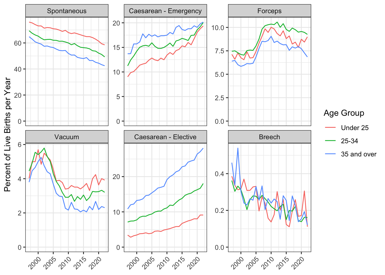

Figure 4.1: Percent of live births per year by age group and delivery type.

4.7 Advanced

If you would like to go beyond what we’ve covered in this chapter, we recommend the following Advanced appendices that are related to this chapter:

• Advanced: Table Formatting (Appendix G)
• Advanced: Data Import (Appendix C)
• Advanced: Data Types (Appendix D)

4.8 Peer Coding Exercises

If you’re enrolled on PSYCH1012 Applied Data Skills, do not do these exercises until the Tuesday workshop.

• The Driver operates the keyboard, implements the next small step, narrates what they are doing.

• The Navigator reviews in real time, thinks ahead, checks naming, design, and help pages, and catches mistakes and typos.

For the final step in this chapter, we will create a report of data visualisations. You may need to refer back to Chapter 2) to help you complete these exercises. We’d also recommend you render at every step so that you can see how your output changes.

TipActivity

There are no solutions provided for the pair programming activities. Everything you need is covered in this book so use the search function and work together to solve any problems.

1. Decide who is going to start as the Driver and Navigator. Remember to switch every so often! The Navigator will find it helpful to have a copy of these instructions open and read the next step to the Driver.

2. Create a copy of the Quarto document that you produced whilst working through this chapter and edit it to present the above code with nice formatting. For example, add headings, hide the code from the output, format the tables, and add in explanations where necessary.

3. Explore the data and add at least one unique insight of your own to the report. You’ll do this for the summative report so it’s good practice. A good place to start is by reviewing the variables in the dataset and trying to think of questions you might want to ask, and answer, of this dataset.

4. Download a different data set from Scottish Health and Social Care Open Data. Create at least one summary tables and one plot of the data and describe that it shows.

Glossary

term	definition
categorical	Data that can only take certain values, such as types of pet.
character	A data type representing strings of text.
csv	Comma-separated variable: a file type for representing data where each variable is separated from the next by a comma.
double	A data type representing a real decimal number
mean	A descriptive statistic that measures the average value of a set of numbers.
median	The middle number in a distribution where half of the values are larger and half are smaller.
pipe	A way to order your code in a more readable format using the symbol %>%
render	To create a file (usually an image or PDF) or widget from source code
vector	A type of data structure that collects values with the same data type, like T/F values, numbers, or strings.

Further resources

• Data transformation cheat sheet
• Chapter 3: Data Transformation in R for Data Science