17 P
17.1 p-value
The probability of seeing an effect at least as extreme as what you have, if the real effect was the value you are testing against (e.g., a null effect)
For example, if you used a binomial test to test against a chance probability of 1/2 (e.g., the probability of heads when flipping a fair coin), then a p-value of 0.37 means that you could expect to see effects at least as extreme as your data (i.e., 55 or more heads or tails) 37% of the time just by chance alone.
# test how likely 55 heads (or a more extreme value)
# is to result from 100 flips of a fair (prob = 0.5) coin
binom.test(55, 100, 0.5)
#>
#>  Exact binomial test
#>
#> data:  55 and 100
#> number of successes = 55, number of trials = 100, p-value =
#> 0.3682
#> alternative hypothesis: true probability of success is not equal to 0.5
#> 95 percent confidence interval:
#>  0.4472802 0.6496798
#> sample estimates:
#> probability of success
#>                   0.55
P-values can be one-tailed or two-tailed. The example above if two-tailed because we didn't specify a direction and are testing whether there were more or fewer heads than expected by chance with a fair coin. The example below is one-tailed, and indicates that you have an 18% chance of getting 55 or more heads when flipping a fair coin 100 times.
# test how likely 55 (or more) heads
# is to result from 100 flips of a fair (prob = 0.5) coin
binom.test(55, 100, 0.5, alternative = "greater")
#>
#>  Exact binomial test
#>
#> data:  55 and 100
#> number of successes = 55, number of trials = 100, p-value =
#> 0.1841
#> alternative hypothesis: true probability of success is greater than 0.5
#> 95 percent confidence interval:
#>  0.4628896 1.0000000
#> sample estimates:
#> probability of success
#>                   0.55
You can see that the p-value is half of the two-tailed value; this is true for symmetric distributions like the binomial distribution, but not for all distributions.
If you do a one-tailed test using "less", the p-value is much higher, indicating that you have an 86% chance of getting 55 or fewer heads when flipping a fair coin 100 times.
# test how likely 55 (or fewer) heads
# is to result from 100 flips of a fair (prob = 0.5) coin
binom.test(55, 100, 0.5, alternative = "less")
#>
#>  Exact binomial test
#>
#> data:  55 and 100
#> number of successes = 55, number of trials = 100, p-value =
#> 0.8644
#> alternative hypothesis: true probability of success is less than 0.5
#> 95 percent confidence interval:
#>  0.0000000 0.6348377
#> sample estimates:
#> probability of success
#>                   0.55
17.2 package
A group of R functions.
Many useful functions are built into R and available by default whenever you start it up. But some of the most powerful things you can do with R require packages of functions that are written by the community. The functions in these packages aren't available until you install the package (using install.packages("package_name") or clicking Install on the Packages pane; this only needs to be done if the package isn't already installed). Once that package is installed (kind of like downloading an app to your phone), you can use it in any script by loading that package as a library at the top of your script (e.g., (library(ggplot2)).
You can alternatively type the package name and two colons before any function from that package to use it without loading all of its functions into the library (e.g., ggplot2::geom_histogram()). This sort of notation is also used to disambiguate function names if two packages have functions with the same names.
17.3 pandoc
A universal document convertor, used by R to make PDF or Word documents from R Markdown
17.4 panes
RStudio is arranged with four window "panes".
By default, the upper left pane is the source pane, where you view and edit source code from files. The bottom left pane is usually the console pane, where you can type in commands and view output messages You can change the location of panes and what tabs are shown under Preferences > Pane Layout.
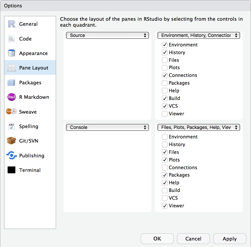
Figure 17.1: Pane layout
17.5 parameter
A quantity characterizing a population.
Often parameters describe a population distribution, such as its mean or SD. They are typically unknown, and therefore must be estimated from the data.
17.6 partial effects
The difference in the response variable for a given change in one predictor variable, with all other covariates held constant.
Also called marginal effects (see this entry for more details).
17.7 partial eta squared
A measure of effect size commonly used in ANOVAs
It measures the proportion of variance explained by a specific independent variable after accounting for variance explained by other variables in the model. It can range from 0 (explains no variance) to 1 (explains 100% of the variance).
The formula for partial eta squared is:
\(\eta_p^2 = SS_{effect} / (SS_{effect} + SS_{error})\)
- \(SS_{effect}\): The sum of squares of for the target effect
- \(SS_{error}\): The sum of squares error in the ANOVA
More...
In the example below, we'll simulate data with significant main effects and an interaction.
# simulate some factorial data
set.seed(8675309)
simdat <- faux::sim_design(
  n = 100,
  within = list(time = c("pre", "post")),
  between = list(treatment = c("control", "experimental")),
  mu = c(100, 105, 100, 110),
  sd = 10,
  r = 0.5,
  id = "ID",
  dv = "DV",
  long = TRUE
)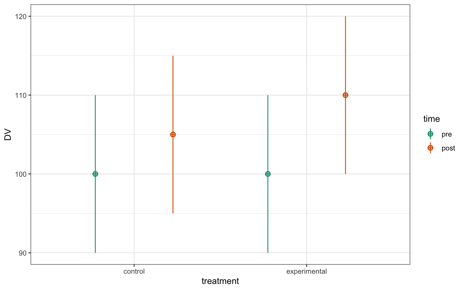
Figure 17.2: CAPTION THIS FIGURE!!
The afex package defaults to generalised eta squared, so you have to set the reported effect size to "pes" to get partial eta squared.
# analysis with ANOVA

library(afex) # a useful package for anova

# set effect size measure to partial eta squared
afex::afex_options(es_aov = "pes")

anova <- afex::aov_ez(
  id = "ID",
  dv = "DV",
  between = "treatment",
  within = "time",
  data = simdat
)
#> Contrasts set to contr.sum for the following variables: treatment

afex::nice(anova)| Effect | df | MSE | F | pes | p.value |
|---|---|---|---|---|---|
| treatment | 1, 198 | 170.45 | 4.63 * | .023 | .033 |
| time | 1, 198 | 56.71 | 109.59 *** | .356 | <.001 |
| treatment:time | 1, 198 | 56.71 | 11.85 *** | .056 | <.001 |
17.8 path
A string representing the location of a file or directory.
A file path can be relative to the working directory or absolute.
# list all files in the images directory,
# use relative path
list.files(path = "images/")
# list all files on the Desktop,
# use absolute path
list.files(path = "/Users/myaccount/Desktop/")
17.9 pipe
A way to order your code in a more readable format using the symbol %>%
The symbol %>% takes the object created by a function and sends it to the next function. By default, it will be used as the first argument, and most tidyverse functions are optimised for this, but you can also include the result as another argument using . (see the example below).
Instead of making a new object for each step:
# this makes 4 unnecessary objects
data <- rnorm(20)         # simulate 20 values
t <- t.test(data)         # 1-sample t-test
p <- t$p.value            # extract p-value
rounded_p <- round(p, 3)  # round to 3 digits
paste("p = ", rounded_p)  # format
#> [1] "p =  0.363"
Or nesting functions:
# this is unreadable; never do this
paste("p = ", round(t.test(rnorm(20))$p.value, 3))
#> [1] "p =  0.363"
You can pipe the results of each function to the next function:
rnorm(20) %>%         # simulate 20 values
  t.test() %>%        # 1-sample t-test
  `[[`("p.value") %>% # extract p-value, `[[`(data, "x") is the same as data[["x"]]
  round(3) %>%        # round to 3 digits
  paste("p = ", .)    # format
#> [1] "p =  0.363"
                      # use . to represent the previous data if it's not the first argument
See a more detailed example.
The symbol | is also called a "pipe" and means "OR" in R, although it has other meanings that are more similar to the %>% pipe in some other programming languages.
17.10 Poisson distribution
A distribution that models independent events happening over a unit of time
lambda <- 3 # mean number of events
x <- rpois(10000, lambda)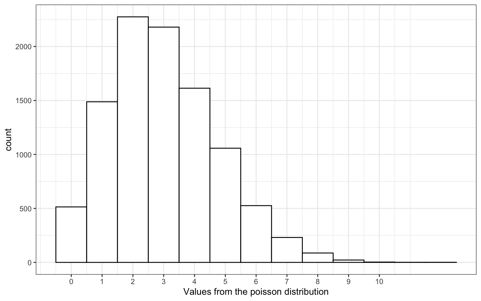
Figure 17.3: Poisson Distribution
17.11 population parameter
A quantity representing a property of a population of interest.
In a psychology context, parameters are constants that are assumed to reflect a typical values for some property appearing in some human group to which we want to generalized. For instance, it may reflect an overall reaction time or an overall priming effect, with individual subjects varying from this fixed value. Population parameters are typically unobserved and usually unobservable due to sampling error and measurement error, and are estimated from the values in the sample. The exception is in data simulation, where hypothetical population parameters can be fixed by the researcher.
17.12 population
All members of a group that we wish to generalise our findings to. E.g. all students taking Psychology at the University of Glasgow. We draw our testing sample from the population..
The population of interest can be any group and it is important that you define this in your study when considering the generalisability of your tests and how you will conduct your sampling. If you want to generalise to everyone in the world then that is the population you should sample from. If you want to generalise to everyone taking Psychology at the University of Glasgow then those are the people you should specifically sample from.
Remember that populations don't have to be humans but could refer to all possible variations of a face for example. The key question is who or what do your results generalise to.
For an interesting paper on populations, samples and generalisability, see:
17.13 power
The probability of rejecting the null hypothesis when it is false.
Formally, the probability of rejecting the null hypothesis, when the null hypothesis is false. Informally, the likelihood of successfully detecting an effect that is actually there (Baguley, 2004). In its simplest application, there is a relationship between alpha, power, effect size, and sample size. This means we can calculate power if we know alpha, the effect size, and the sample size. This would tell us -- in the long run -- how many times would I observe a significant effect for a given alpha, effect size, and sample size?
More...
For example, you can simulate a 2-sample study 100 times, where the true mean for group A is 100 and the true mean for group B is 105, and the SD for each group is 10.
set.seed(8675309) # for reproducible simulations

sim_data <- faux::sim_design(
  between = list(group = c("A", "B")),
  n = c(A = 50, B = 45), # number of subjects per group
  mu = c(A = 100, B = 105),
  sd = 10,
  rep = 100, # repeat the simulation 100 times
  long = TRUE, # structure data in long format
  plot = FALSE
)
Now you can use iteration to run your analysis on each sample, saving the p-value.
p_values <- purrr::map_dbl(sim_data$data, function(data) {
  t.test(y ~ group, data = data)$p.value
})
Finally, check what proportion of the samples resulted in a significant p-value. This is your power.
alpha <- 0.05 # justify your alpha
power <- mean(p_values < alpha)
power
#> [1] 0.7
17.14 predictor variable
A variable whose value is used (in a model) to predict the value of a response variable.
In an experimental context, predictor variables are often referred to as independent variables.
17.15 preregistration
Specifying the methods and analysis of a study before it is run.
Resources:
- Center for Open Science
- The Preregistration Revolution: PNAS / Preprint
17.16 probability
A number between 0 and 1 where 0 indicates impossibility of the event and 1 indicates certainty
See also probability distribution.
17.17 project
A way to organise related files in RStudio.
Choose New Project... under the File menu to create a new project in a new folder, organise an existing folder of files as a project, or download a version controlled repository as a project.
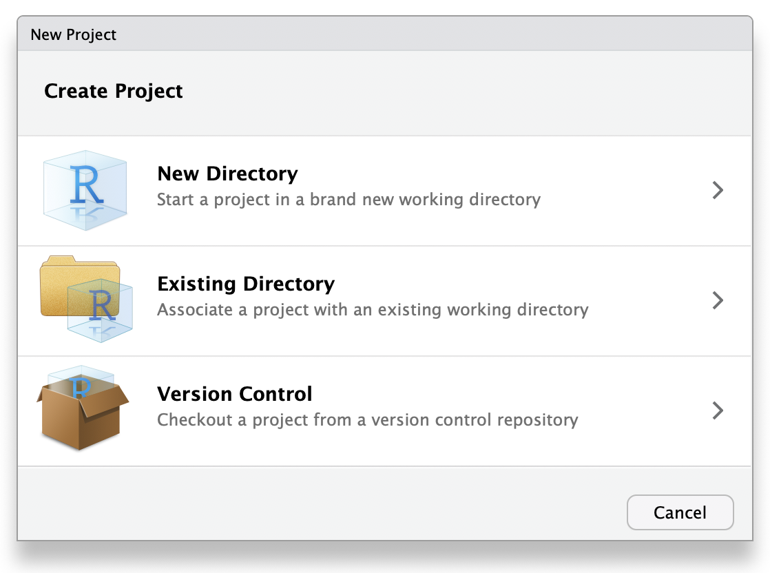
Figure 17.4: Start a new project
17.18 pseudoreplication
The process of artificially inflating the number of samples or replicates
Pseudoreplications can occur when you take multiple measurements within the same condition.
For instance, imagine a study where you randomly assign participants to consume one of two beverages—alcohol or water—before administering a simple response time task where they press a button as fast as possible when a light flashes. You would probably take more than one measurement of response time for each participant; let's assume that you measured it over 100 trials. You’d have one between-subject factor (beverage) and 100 observations per subject, for say, 20 subjects in each group.
One common mistake novices make when analyzing such data is to try to run a t-test. You can’t directly use a conventional t-test when you have pseudoreplications (or multiple stimuli). You must first calculate means for each subject, and then run your analysis on the means, not on the raw data. There are versions of ANOVA that can deal with pseudoreplications, but you are probably better off using a linear-mixed effects model, which can better handle the complex dependency structure.