2 A
2.1 absolute path
A file path that starts with / and is not appended to the working directory
For example, if your working directory is /Users/me/study/ and you want to refer to a file in the directory data called faces.csv, the absolute path is /Users/me/study/data/faces.csv.
However, you should normally use relative paths in scripts, not absolute paths, which can change when you move a project directory to a new computer or even a new place on your computer.
The package R.utils has a function getAbsolutePath() that returns the absolute path of a file path or a file object.
caminho absoluto: um caminho para um arquivo que começa com / e não está fixado ao diretório de trabalho
Por exemplo, se o seu diretório de trabalho é /Users/me/study/ e você quer se referir a um arquivo no diretório data chamado faces.csv, o caminho absoluto é /Users/me/study/data/faces.csv.
Entretanto, você deve normalmente usar caminhos relativos nos scripts, não caminhos absolutos, pois estes podem mudar quando você move o diretório de um projeto para um computador novo ou até mesmo para um destino novo no seu computador.
O pacote R.utils possui uma função getAbsolutePath() que retorna o caminho absoluto de um arquivo caminho ou um arquivoobjeto
R.utils::getAbsolutePath("../index.Rmd")
#> [1] "/Users/debruine/rproj/psyteachr/index.Rmd"
2.2 adjusted R-squared
A modified version of R-squared adjusted for the number of predictors in the model.
R-quadrado ajustado: uma versão modificada do R-quadrado ajustado para o número de preditores do modelo.
2.3 alpha
(stats) The cutoff value for making a decision to reject the null hypothesis; (graphics) A value between 0 and 1 used to control the levels of transparency in a plot
Can also be a parameter in the beta distribution or refer to Cronbach's alpha.
(stats) alfa: o valor limite para tomar uma decisão ao rejeitar uma hipótese nula; graphics) um valor entre 0 e 1 usado para controlar os níveis de transparência em um gráfico
Pode ser também um parâmetro na distribuição beta beta distribution ou se referir ao alfa de Cronbach Cronbach's alpha.
2.4 alpha (stats)
The cutoff value for making a decision to reject the null hypothesis
If you are using null hypothesis significance testing (NHST), then you need to decide on a cutoff value called alpha for making a decision to reject the null hypothesis. We call p-values below the alpha cutoff significant.
In psychology, alpha is traditionally set at \(\alpha\) = .05, but there are good arguments for setting a different criterion in some circumstances.
alfa: o valor limite para tomar uma decisão ao rejeitar uma hipótese nula
alfa (estatística): se você estiver usando o teste de significância da hipótese nula, você deve decidir um limiar de valor chamado alfa para tomar uma decisão sobre rejeitar a hipótese nula. P-valores abaixo do limiar do alfa são chamados de significativos.
Na psicologia, o alfa é tipicamente estabelecido como \(\alpha\) = .05, mas há bons argumentos para estabelecer um critério diferente em algumas circunstâncias.
2.5 alpha (graphics)
A value between 0 and 1 used to control the levels of transparency in a plot
Um valor entre 0 e 1 usado para controlar os níveis de transparência em um gráfico
More...
# if you omit alpha, it defaults to 1
alpha1.00 <- ggplot(diamonds, aes(x = depth, fill = cut)) +
  geom_density() + xlim(55, 70)

alpha0.25 <- ggplot(diamonds, aes(x = depth, fill = cut)) +
  geom_density(alpha = 0.25) + xlim(55, 70)

cowplot::plot_grid(alpha1.00, alpha0.25, nrow = 2,
                   labels = c("alpha = 1.0", "alpha = 0.25"))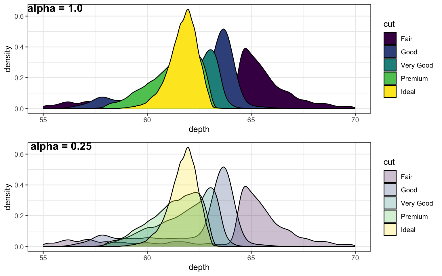
Figure 2.1: Setting alpha to a number lower than 1 lets you see parts of the plot hidden behind an object.
2.6 alternate hypothesis
The hypothesis that an observed difference between groups or from a specific value is NOT due to chance alone.
The alternate hypothesis is also commonly referred to as H1. This is contrasted with H0, the null hypothesis in a null hypothesis significance testing (NHST) framework.
2.7 ampersand
The symbol &, an operator meaning "AND".
A single ampersand is vectorized, so compares each item in the first vector with the corresponding item in the second vector.
A double ampersand is not vectorised, so will ignore all but the first item in vectors, unless you have set the environment variable _R_CHECK_LENGTH_1_LOGIC2_ to true, in which case you will get an error.
Sys.setenv("_R_CHECK_LENGTH_1_LOGIC2_" = "false")
c(T, T, F, F) && c(T, T, F, F)
#> Error in c(T, T, F, F) && c(T, T, F, F): 'length = 4' in coercion to 'logical(1)'
Sys.setenv("_R_CHECK_LENGTH_1_LOGIC2_" = "true")
c(T, T, F, F) && c(T, T, F, F)
#> Error in c(T, T, F, F) && c(T, T, F, F): 'length = 4' in coercion to 'logical(1)'
The advantage of a double ampersand is that it will stop as soon as the conclusion is obvious. So if the first item is FALSE, the second item won't even be run. This is useful for testing whether an object exists before checking something that requires the object to exist.
# this produces an error if x doesn't exist
if (is.character(x)) {
  # do something
}
#> Error in eval(expr, envir, enclos): object 'x' not found
if (exists("x") && is.character(x)) {
  # do something
}
2.8 ancova
ANalysis of CO-VAriance: a type of linear model that is useful for factorial designs with continuous covariates
See also ANOVA.
More...
# simulate some factorial data
set.seed(8675309)
simdat <- faux::sim_design(
  n = 100,
  between = list(treatment = c("control", "experimental")),
  mu = c(100, 105),
  sd = 10,
  id = "ID",
  dv = "DV",
  plot = FALSE
)

# add a covariate that is correlated r = 0.5 to the DV
simdat$cov <- faux::rnorm_pre(simdat$DV, mu = 0, sd = 1, r = 0.5)

head(simdat)| ID | treatment | DV | cov |
|---|---|---|---|
| S001 | control | 90.03418 | -0.5848813 |
| S002 | control | 107.21824 | 1.2256043 |
| S003 | control | 93.82791 | -0.5048147 |
| S004 | control | 120.29392 | 0.4131685 |
| S005 | control | 110.65416 | 0.3075864 |
| S006 | control | 109.87220 | 1.2536715 |
# analysis with ANCOVA

library(afex) # a useful package for ancova

ancova <- afex::aov_ez(
  id = "ID",
  dv = "DV",
  between = "treatment",
  covariate = "cov",
  factorize = FALSE, # must be FALSE with covariates
  data = simdat
)
#> Warning: Numerical variables NOT centered on 0 (matters if variable in interaction):
#>    cov
#> Contrasts set to contr.sum for the following variables: treatment

afex::nice(ancova)| Effect | df | MSE | F | ges | p.value |
|---|---|---|---|---|---|
| treatment | 1, 197 | 69.80 | 9.03 ** | .044 | .003 |
| cov | 1, 197 | 69.80 | 64.72 *** | .247 | <.001 |
2.9 ANOVA
ANalysis Of VAriance: a type of linear model that is useful for factorial designs
See also ANCOVA.
More...
# simulate some factorial data
set.seed(8675309)
simdat <- faux::sim_design(
  n = 100,
  within = list(time = c("pre", "post")),
  between = list(treatment = c("control", "experimental")),
  mu = c(100, 100, 100, 105),
  sd = 10,
  r = 0.5,
  id = "ID",
  dv = "DV",
  long = TRUE
)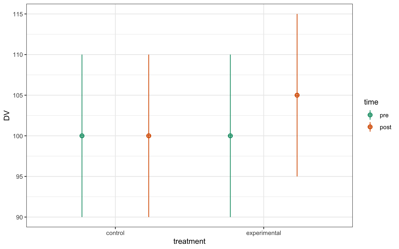
Figure 2.2: 2x2 factorial data
# analysis with ANOVA

library(afex) # a useful package for anova

anova <- afex::aov_ez(
  id = "ID",
  dv = "DV",
  between = "treatment",
  within = "time",
  data = simdat
)
#> Contrasts set to contr.sum for the following variables: treatment

afex::nice(anova)| Effect | df | MSE | F | ges | p.value |
|---|---|---|---|---|---|
| treatment | 1, 198 | 170.45 | 4.63 * | .017 | .033 |
| time | 1, 198 | 56.71 | 14.66 *** | .018 | <.001 |
| treatment:time | 1, 198 | 56.71 | 11.85 *** | .015 | <.001 |
2.10 anti_join
A filtering join that returns all rows from the left table where there are not matching values in the right table, keeping just columns from the left table.
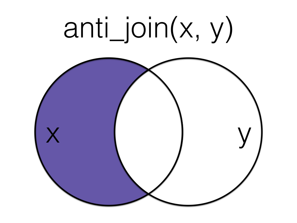
Figure 2.3: Anti Join
This is useful when you have a table of data that contains IDs you want to exclude from your main dataset.
all_data <- tibble(
  id = 1:5,
  x = LETTERS[1:5]
)

to_exclude <- tibble(
  id = 2:4
)

data <- anti_join(all_data, to_exclude, by = "id")| id | x |
|---|---|
| 1 | A |
| 5 | E |
See joins for other types of joins and further resources.
2.11 argument
A variable that provides input to a function.
For example, the first argument to the function rnorm() is n (the number of observations).
When you look up the help for a function (e.g., ?sd), you will see a section called Arguments, which lists the argument names and their definitions.
The function args() will show you the argument names and their default values (if any) for any function.
args(rnorm)
#> function (n, mean = 0, sd = 1)
#> NULL
2.12 array
A container that stores objects in one or more dimensions.
You can create an array by specifying a list or vector of values and the number of dimensions. The first two dimensions are rows and columns; each dimension after that is printed separately as a facet.
# 3-dimensional array with 4 rows, 3 columns, and 2 facets
array(1:24, dim = c(4, 3, 2))
#> , , 1
#>
#>      [,1] [,2] [,3]
#> [1,]    1    5    9
#> [2,]    2    6   10
#> [3,]    3    7   11
#> [4,]    4    8   12
#>
#> , , 2
#>
#>      [,1] [,2] [,3]
#> [1,]   13   17   21
#> [2,]   14   18   22
#> [3,]   15   19   23
#> [4,]   16   20   24
More...
You can give your array dimensions names.
dimnames <- list(
  subj_id = c("S1", "S2", "S3", "S4"),
  face_id = c("F1", "F2", "F3"),
  condition = c("Control", "experimental")
)

array(1:24, dim = c(4, 3, 2), dimnames = dimnames)
#> , , condition = Control
#>
#>        face_id
#> subj_id F1 F2 F3
#>      S1  1  5  9
#>      S2  2  6 10
#>      S3  3  7 11
#>      S4  4  8 12
#>
#> , , condition = experimental
#>
#>        face_id
#> subj_id F1 F2 F3
#>      S1 13 17 21
#>      S2 14 18 22
#>      S3 15 19 23
#>      S4 16 20 24
Objects not need to be the same data type.
2.13 aspect ratio
The ratio between the width and height of an image.
You can specify the aspect ratio of your plots by setting the width and height in the first chunk of an R Markdown file, in the chunk options, or when you save the image.
More...
Knitr defaults:
knitr::opts_chunk$set(
  fig.width = 7, # default value is 7
  fig.height = 7/1.618 # rolden ratio; default value is 7
)
Chunk options:
```{r fig-golden-ratio, fig.width = 7, fig.height = 4.32}
ggplot(iris, aes(Sepal.Width, Sepal.Length, color = Species)) +
  geom_point() +
  geom_smooth(method = lm, formula = y~x)
```
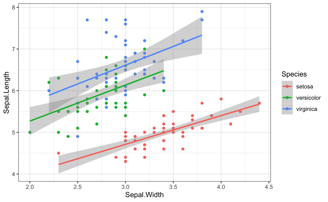
Figure 2.4: Plot with a 1.618:1 aspect ratio (golden ratio)
```{r fig-square, fig.width = 7, fig.height = 7}
ggplot(iris, aes(Sepal.Width, Sepal.Length, color = Species)) +
  geom_point() +
  geom_smooth(method = lm, formula = y~x)
```
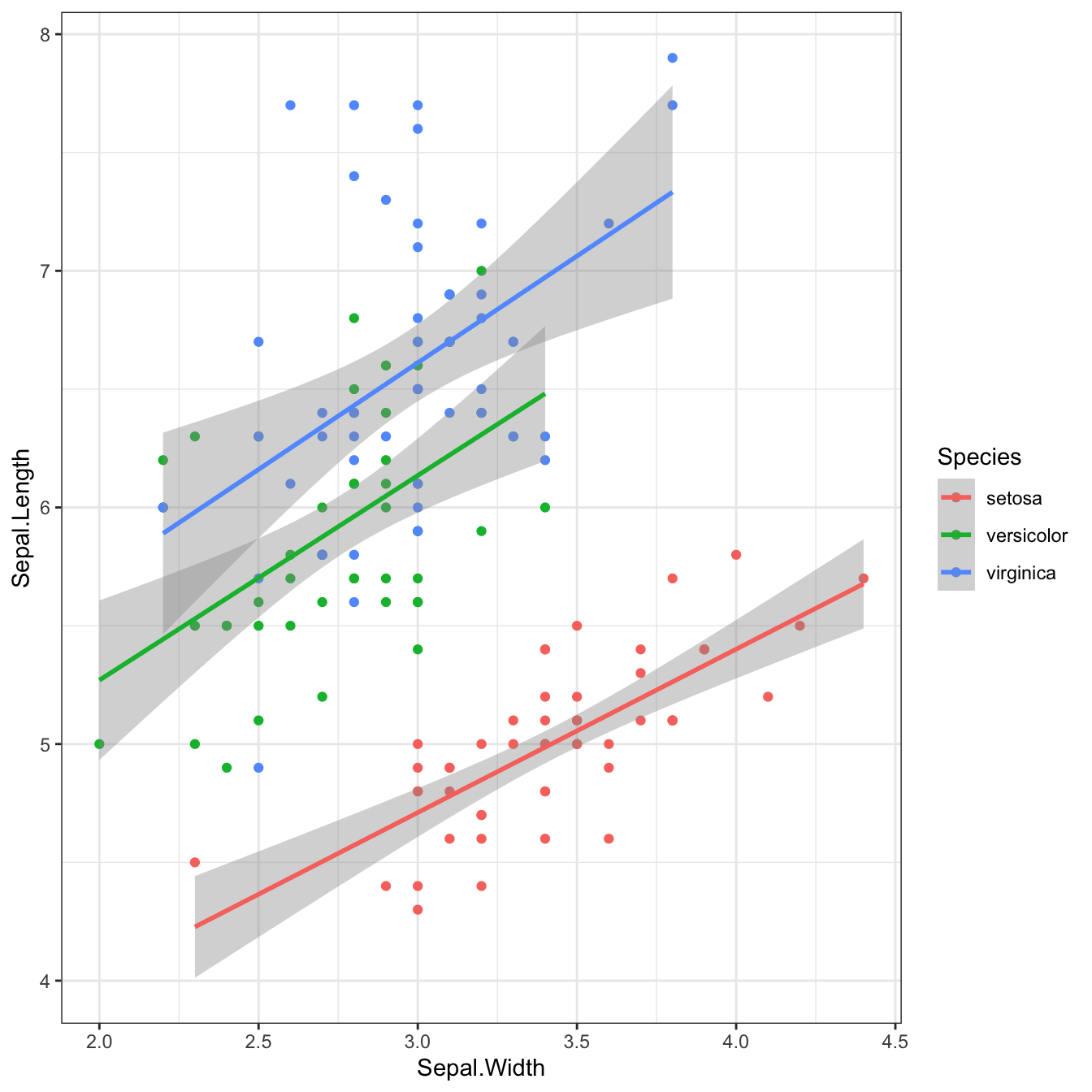
Figure 2.5: Plot with a 1:1 aspect ratio
On save:
ggsave("golden-ratio.jpg", width = 7, height = 7/1.618)2.14 assignment operator
The symbol <-, which functions like = and assigns the value on the right to the object on the left
a <- 1

a
#> [1] 1
The assignment operator can also be reversed
2 -> b

b
#> [1] 2
And even go in both direction at the same time!
x <- 2 -> y

x
#> [1] 2
y
#> [1] 2
2.15 atomic
Only containing objects with the same data type (e.g., all numeric or character).
Vectors are atomic data structures in R.
a <- c(1, 4, 32)
b <- c("somebody", "once", "told me")
class(a)
#> [1] "numeric"
class(b)
#> [1] "character"
More...
If you try to mix data types in an atomic vector, they will be coerced to be the same type. (Note that 32 becomes "32" so it can be in the same vector as a character object).
c(32, TRUE, "eighteen")
#> [1] "32"       "TRUE"     "eighteen"
Another feature of vectors that makes them atomic is that they are always flat. If you embed vectors within vectors, they will be flattened.
Lists, on the other hand, can be nested.
list(7, c(1, 4, 32), 2, 6) %>% str()
#> List of 4
#>  $ : num 7
#>  $ : num [1:3] 1 4 32
#>  $ : num 2
#>  $ : num 6
If you try to extract objects inside an atomic vector, you need to use brackets []. This can be with an index or a name. Single brackets can return one or more elements, and include names, while double brackets can only return one element and don't have names.
my_vec <- c(x = 3, y = 1, z = 4)
my_vec[2]
#> y
#> 1
my_vec["y"]
#> y
#> 1
my_vec[["y"]]
#> [1] 1
You cannot use the $ operator on an atomic vector, or you will get this very common error.
my_vec$y
#> Error in my_vec$y: $ operator is invalid for atomic vectors
See the Vectors chapter of Advanced R for more advanced discussion of atomic vectors.
2.16 attribute
Extra information about an R object
You can access an object's attributes with attr(). For example, datasets simulated with faux have an attribute called "design" that details their design.
data <- faux::sim_design(
  between = list(pet = c(cat = "Cat Owners",
                         dog = "Dog Owners")),
  within = list(time = c(am = "Morning",
                         pm = "Night")),
  mu = 1:4,
  r = list(cat = 0.3, dog = 0.6),
  dv = c(score = "Happiness Scale Score"),
  plot = FALSE)

design <- attr(data, "design")

design$dv
#> $score
#> [1] "Happiness Scale Score"
2.17 attribute (html)
Extra information about an HTML element
For example, the paragraph element has an attribute of "id" with a value of "feature". This can be used to refer to the element to change its style with CSS or affect its behaviour with JavaScript.