18 Q

18.1 Q-Q plot

A scatterplot created by plotting two sets of quantiles against each other, used to check if data come from a specified distribution

It is pretty difficult to tell from looking at a density plot if data are distributed in a specific way. We often want to determine if, for example, the residuals of a model are normally distributed. Q-Q plots can help with this.

More...

Let's simulate 25 data points from a normal distribution with a mean of 100 and SD of 10. Since there are not many data points, the resulting plot will be pretty lumpy. The red line is a perfect normal distribution.

set.seed(8675309) # for reproducible random values

A <- rnorm(25, 100, 10)

ggplot() + 
  geom_density(aes(A)) +
  geom_function(fun = dnorm, 
                args = list(mean = 100, sd = 10),
                colour = "red")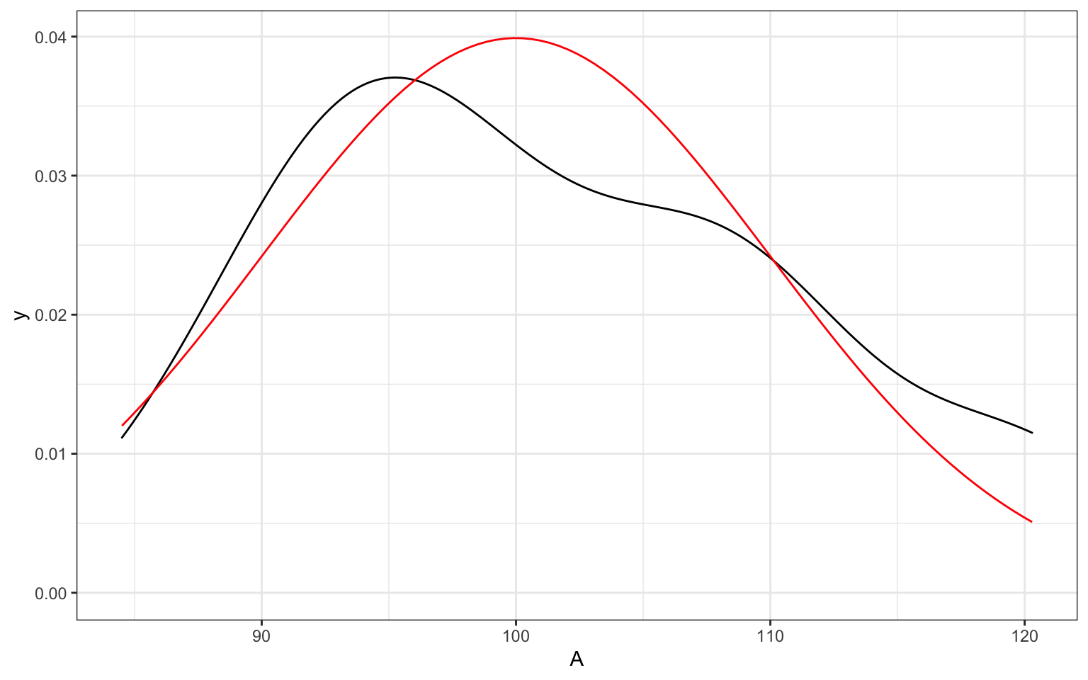

Figure 18.1: Density plot of sample data and the normal distribution it was drawn from

A Q-Q plot calculates what quantile each data point is in, and plots that against the theoretical quantiles from the normal distribution. The red line is the theoretically perfect noraml distribution, so you just need to assess if most of the points fall on this line.

qplot(sample = A) + geom_qq_line(colour = "red")

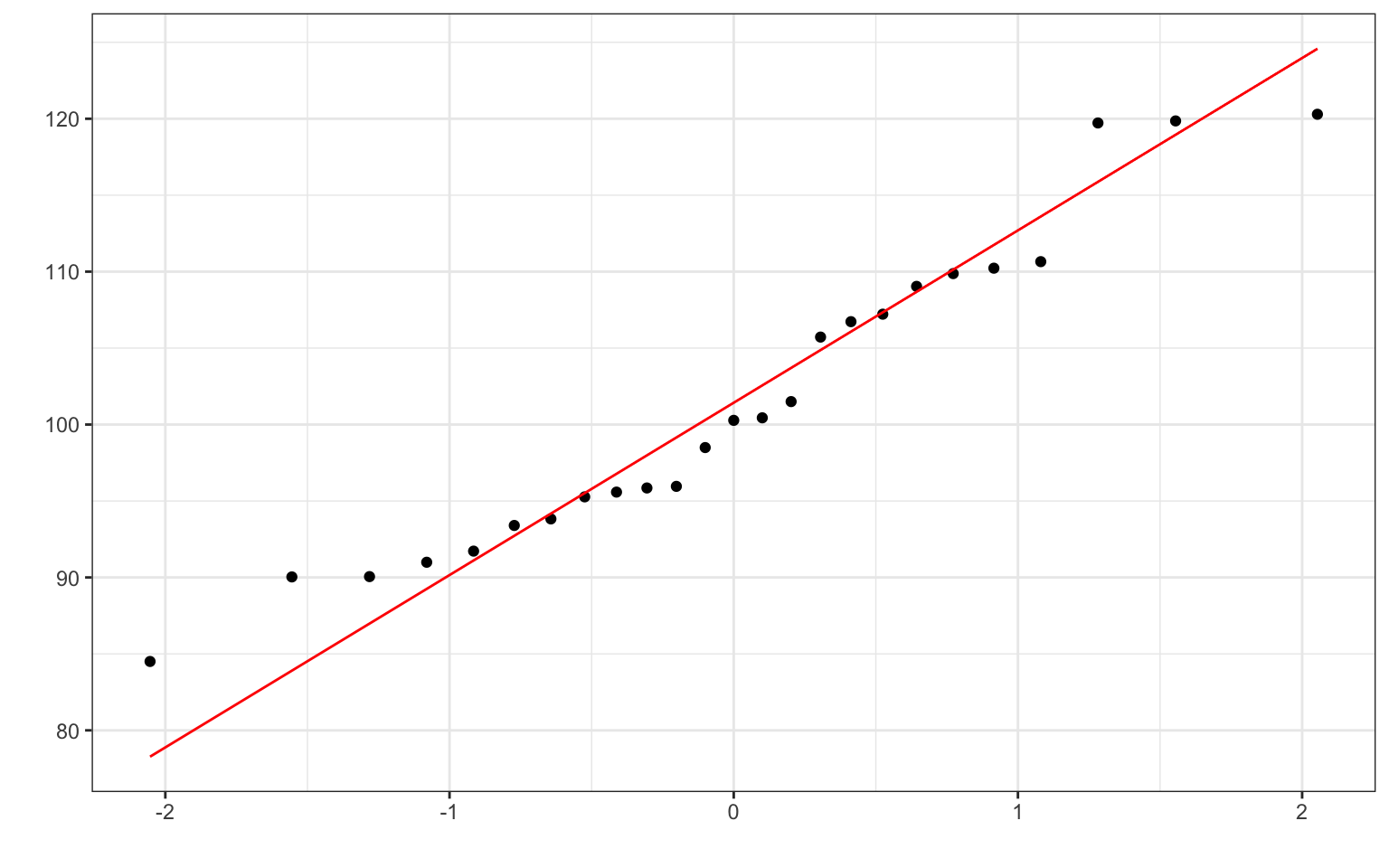
Figure 18.2: Q-Q plot of a small sample from a normal distribution

Here's what it might look like if your data are actually from a uniform distribution.

U <- runif(25, 0, 10)
qplot(sample = U) + geom_qq_line(colour = "red")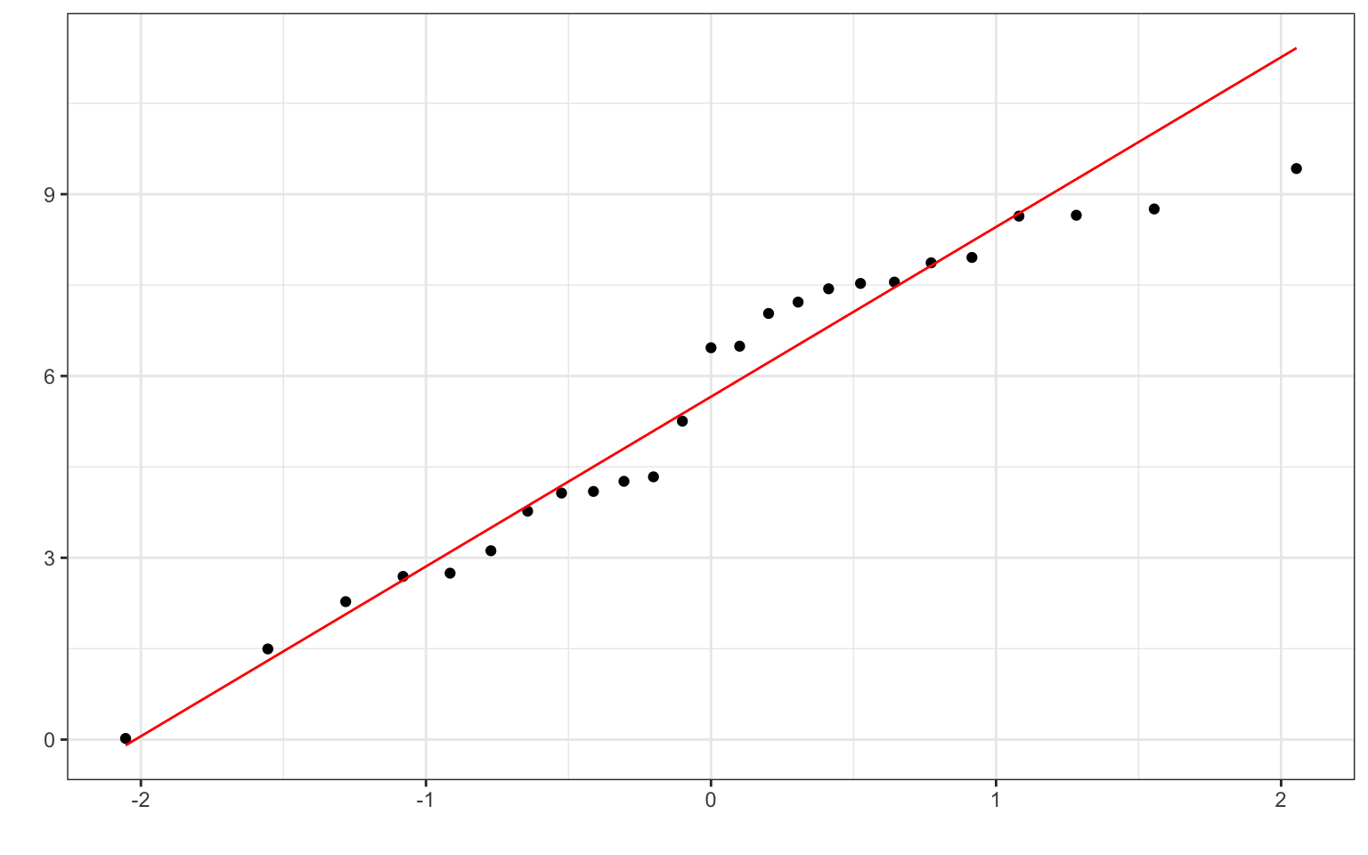

Figure 18.3: Q-Q plot of a uniform distribution

18.2 quantile

Cutoffs dividing the range of a distribution into continuous intervals with equal probabilities.

More...

You can take a sample of numbers on divide them into N equally-sized groups. Let's use these 12 numbers as an example:

x <- c(1, 1, 2, 2, 3, 4, 4, 5, 7, 7, 7, 10)

The quantile() function gives you the cutoffs for each quantile from the data. Set the argument probs to seq(0, 1, 1/N) for any N-tile.

# median
quantile(x, probs = seq(0, 1, 1/2))
#>   0%  50% 100% 
#>    1    4   10

# tertile
quantile(x, probs = seq(0, 1, 1/3))
#>        0% 33.33333% 66.66667%      100% 
#>  1.000000  2.666667  5.666667 10.000000

# quartile
quantile(x, probs = seq(0, 1, 1/4))
#>   0%  25%  50%  75% 100% 
#>    1    2    4    7   10

dat <- data.frame(
  x = x
) %>%
  mutate(
  `2-tile` = ntile(x, 2),
  `3-tile` = ntile(x, 3),
  `4-tile` = ntile(x, 4),
  `6-tile` = ntile(x, 6)
)

x	2-tile	3-tile	4-tile	6-tile
1	1	1	1	1
1	1	1	1	1
2	1	1	1	2
2	1	1	2	2
3	1	2	2	3
4	1	2	2	3
4	2	2	3	4
5	2	2	3	4
7	2	3	3	5
7	2	3	4	5
7	2	3	4	6
10	2	3	4	6

See Q_Q plots.