6 Clean Water and Sanitation
![]()
Ensure availability and sustainable management of water and sanitation for all
6.1 Original Data
WHO/UNICEF Joint Monitoring Programme for Water Supply, Sanitation and Hygiene (JMP) (2024) – with major processing by Our World in Data)
Codebook
- Entity: Country
- Code: 3-letter ISO country code
- Year
- Share of the population using safely managed drinking water services: safe
- Share of the population using only basic drinking water services: basic
- Share of the population using limited drinking water services: limited
- Share of the population using unimproved drinking water services: unimproved
- Share of the population using surface water as a primary source of drinking water: surface
6.2 Simplified Subsets
6.2.1 Long Countries
A data set with long structure and short column names consistent with other data sets in this book, limited to individual countries.
Code
access_levels <- c("safe", "basic", "limited", "unimproved", "surface")

water_countries <- read_csv(
  "data/06/access-drinking-water/access-drinking-water-stacked.csv",
  col_names = c("country_name", "country_code", "year", access_levels),
  skip = 1, show_col_types = FALSE
) |>
  filter(!is.na(country_code)) |>
  pivot_longer(safe:surface, names_to = "access", values_to = "pcnt") |>
  mutate(access = factor(access, access_levels),
         pcnt = round(pcnt, 2),
         country_code = gsub("OWID_", "", country_code))
This set is good for dealing with categorical columns with a clear order that isn’t the default on import.
| country_name | country_code | year | access | pcnt |
|---|---|---|---|---|
| Afghanistan | AFG | 2000 | safe | 11.09 |
| Afghanistan | AFG | 2000 | basic | 16.35 |
| Afghanistan | AFG | 2000 | limited | 3.30 |
| Afghanistan | AFG | 2000 | unimproved | 43.86 |
| Afghanistan | AFG | 2000 | surface | 25.40 |
| Afghanistan | AFG | 2001 | safe | 11.11 |
Code
access_col <- c("#26BDE2", "#4C9F38", "#DDA63A", "#FD6925", "#DD1367")

water_countries |>
  # narorw to complete entries
  filter(year == 2022) |>
  #filter(sum(pcnt) > 99, .by = c(country_name)) |>
  mutate(quantile = case_when(row_number()<= n()/4 ~ 1,
                              row_number()<= 2*n()/4 ~ 2,
                              row_number()<= 3*n()/4 ~ 3,
                              .default = 4)) |>
  ggplot(aes(x = fct_rev(country_code), y = pcnt, fill = access)) +
  facet_wrap(~quantile, scales = "free", ncol = 4) +
  geom_col() +
  coord_flip() +
  scale_fill_manual(values = access_col) +
  labs(x = NULL, y = NULL) +
  theme(legend.position = "top",
        strip.background = element_blank(),
        strip.text = element_blank())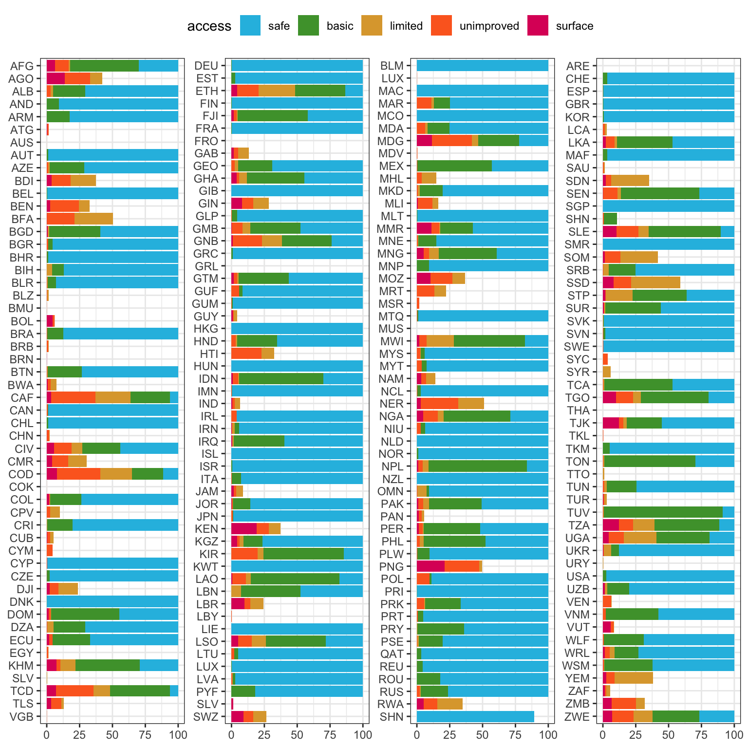
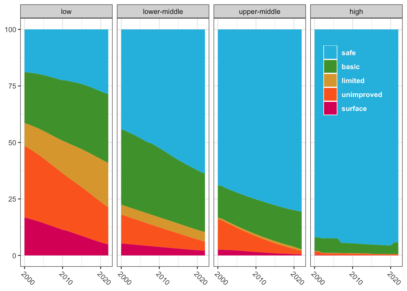
6.2.2 Water Regions
The data are also grouped by WHO and SDG regions, and by development levels. This set includes just those regions, with region_type as the grouping (WHO, SDG, DEV).
Code
access_levels <- c("safe", "basic", "limited", "unimproved", "surface")

water_regions <- read_csv(
  "data/06/access-drinking-water/access-drinking-water-stacked.csv",
  col_names = c("region_name", "country_code", "year", access_levels),
  skip = 1, show_col_types = FALSE
) |>
  filter(is.na(country_code), region_name != "Bonaire, Sint Eustatius and Saba") |>
  select(-country_code) |>
  pivot_longer(safe:surface, names_to = "access", values_to = "pcnt") |>
  mutate(access = factor(access, access_levels),
         pcnt = round(pcnt, 2)) |>
  separate(region_name, c("region", "region_type"), sep = "\\(|\\)", extra = "drop", fill = "right") |>
  mutate(region_type = replace_na(region_type, "DEV"),
region = trimws(region))| region | region_type | year | access | pcnt |
|---|---|---|---|---|
| Africa | WHO | 2000 | safe | 19.31 |
| Africa | WHO | 2000 | basic | 28.48 |
| Africa | WHO | 2000 | limited | 8.81 |
| Africa | WHO | 2000 | unimproved | 25.89 |
| Africa | WHO | 2000 | surface | 17.50 |
| Africa | WHO | 2001 | safe | 19.61 |
Code
region_names <- c("Low-income countries",
                  "Lower-middle-income countries",
                  "Upper-middle-income countries",
                  "High-income countries")
region_labels <- c("low", "lower-middle", "upper-middle", "high")
access_col <- c("#26BDE2", "#4C9F38", "#DDA63A", "#FD6925", "#DD1367")

water_regions |>
  filter(grepl("income", region)) |>
  mutate(region = factor(region, region_names, region_labels)) |>
  ggplot(aes(x = year, y = pcnt, fill = access)) +
  geom_area() +
  facet_wrap(~region, ncol = 4) +
  scale_x_continuous(breaks = seq(2000, 2020, 10)) +
  scale_fill_manual(values = access_col) +
  guides(fill = guide_legend(position = "inside")) +
  labs(x = NULL, y = NULL, fill = NULL) +
  theme(axis.text.x = element_text(angle = -45, hjust = 0),
        legend.background = element_blank(),
        legend.position.inside = c(.87,.75),
        legend.text = element_text(color = "white", face = "bold"))