10 Advanced Reports
10.1 Intended Learning Outcomes
- Structure data in report, presentation, and dashboard formats
- Include linked figures, tables, and references
library(tidyverse)     # data wrangling functions
library(bookdown)      # for chaptered reports
library(flexdashboard) # for dashboards
library(DT)            # for interactive tables
Download the R Markdown Cheat Sheet.
Until now, we've only used the default html_document output format in an R markdown report, but there are several other output formats that you can try.
10.2 Reports
10.2.1 Word documents
In the YAML header of an R Markdown document, you can change output to word_document to create a Microsoft Word file. Make sure you carefully check your file; images and tables can often look odd or page breaks can happen in strange ways.
You can add page breaks by adding \newpage on a line by itself with blank lines above and below.
10.2.2 PDF documents
If you have a latex installation (see Appendix A), you can create a PDF by setting output to pdf_document.
Note that this can sometimes cause problems with kableExtra tables and you can't use some elements like interactive plots. Additionally, the figures and tables are likely to shift from their position in text to the top or bottom of pages.
See the PDF section of R Markdown: The Definitive Guide (Xie et al., 2018) for more advanced customisation options.
10.2.3 Linked documents
If you need to create longer reports with links between sections, you can use one of the bookdown formats. bookdown::html_document2 is a useful one that adds figure and table numbers automatically to any figures or tables with a caption and allows you to link to these by reference.
Refer to figures and tables like the code below. Figures start with "fig:" and tables with "tab:", then the code chunk name that created the figure or table.
See Table\ \@ref(tab:table-name) or Figure\ \@ref(fig:fig-name).The code chunk names can only contain letters, numbers and dashes. If they contain other characters like spaces or underscores, the referencing will not work.
The code below shows how to link text to figures or tables. You can see the HTML output here.
---
title: "Linked Document Demo"
output:
  bookdown::html_document2:
    number_sections: false
---

```{r setup, include=FALSE}
knitr::opts_chunk$set(echo = FALSE,
                      message = FALSE,
                      warning = FALSE)
library(tidyverse)
library(kableExtra)
theme_set(theme_minimal())
```

Diamond price depends on many features, such as:

- cut (See Table\ \@ref(tab:by-cut))
- colour (See Table\ \@ref(tab:by-colour))
- clarity (See Figure\ \@ref(fig:by-clarity))
- carats (See Figure\ \@ref(fig:by-carat))

## Tables

### Cut

```{r by-cut}
diamonds %>%
  group_by(cut) %>%
  summarise(avg = mean(price),
            .groups = "drop") %>%
  kable(digits = 0,
        col.names = c("Cut", "Average Price"),
        caption = "Mean diamond price by cut.") %>%
  kable_material()
```

### Colour

```{r by-colour}
diamonds %>%
  group_by(color) %>%
  summarise(avg = mean(price),
            .groups = "drop") %>%
  kable(digits = 0,
        col.names = c("Cut", "Average Price"),
        caption = "Mean diamond price by colour.") %>%
  kable_material()
```

## Plots

### Clarity

```{r by-clarity, fig.cap = "Diamond price by clarity"}
ggplot(diamonds, aes(x = clarity, y = price)) +
  geom_boxplot()
```

### Carats

```{r by-carat, fig.cap = "Diamond price by carat"}
ggplot(diamonds, aes(x = carat, y = price)) +
  stat_smooth()
```
This format defaults to numbered sections, so set number_sections: false in the YAML header if you don't want this.
10.2.4 References
There are several ways to do in-text references and automatically generate a bibliography in R Markdown. Markdown files need to link to a BibTex file (a plain text file with references in a specific format) that contains the references you need to cite. You specify the name of this file in the YAML header, like bibliography: filename.bib and cite references in text using an at symbol and a shortname, like [@tidyverse].
10.2.4.1 Creating a BibTeX file
Most reference software like EndNote, Zotero or Mendeley have exporting options that can export to BibTeX format. You just need to check the shortnames in the resulting file.
You can also make a BibTeX file and add references manually. In RStudio, go to File > New File... > Text File and save the file as "bibliography.bib".
Next, add the line bibliography: bibliography.bib to your YAML header.
10.2.4.2 Adding references
You can add references to a journal article in the following format:
@article{shortname,
  author = {Author One and Author Two and Author Three},
  title = {Paper Title},
  journal = {Journal Title},
  volume = {vol},
  number = {issue},
  pages = {startpage--endpage},
  year = {year},
  doi = {doi}
}
See A complete guide to the BibTeX format for instructions on citing books, techincal reports, and more.
You can get the reference for an R package using the functions citation() and toBibtex(). You can paste the bibtex entry into your bibliography.bib file. Make sure to add a short name (e.g., "ggplot2") before the first comma to refer to the reference.
## @Book{,
##   author = {Hadley Wickham},
##   title = {ggplot2: Elegant Graphics for Data Analysis},
##   publisher = {Springer-Verlag New York},
##   year = {2016},
##   isbn = {978-3-319-24277-4},
##   url = {https://ggplot2.tidyverse.org},
## }
Google Scholar entries have a BibTeX citation option. This is usually the easiest way to get the relevant values, although you have to add the DOI yourself. You can keep the suggested shortname or change it to something that makes more sense to you.
10.2.4.3 Citing references
You can cite references in text like this:
This tutorial uses several R packages [@tidyverse;@rmarkdown].This tutorial uses several R packages (Allaire et al., 2018; Wickham, 2017).
Put a minus in front of the @ if you just want the year:
Franconeri and colleagues [-@franconeri2021science] review research-backed guidelines for creating effective and intuitive visualizations.Franconeri and colleagues (2021) review research-backed guidelines for creating effective and intuitive visualizations.
If you want to add an item to the reference section without citing it, add it to the YAML header like this:
nocite: |
  @ref1, @ref2, @ref3
Or add all of the items in the .bib file like this:
nocite: '@*'10.2.4.4 Citation styles
You can search a list of style files (e.g., APA, MLA, Harvard) and download a file that will format your bibliography. You'll need to add the line csl: filename.csl to your YAML header.
10.2.5 Interactive tables
One way to make your reports more exciting is to use interactive tables. The DT::datatable() function displays a table with some extra interactive elements to allow readers to search and reorder the data, as well as controlling the number of rows shown at once. This can be especially helpful. This only works with HTML output types. The DT website has extensive tutorials, but we'll cover the basics here.
library(DT)

scotpop <- read_csv("data/scottish_population.csv",
                    show_col_types = FALSE)

datatable(data = scotpop)
You can customise the display, such as changing column names, adding a caption, moving the location of the filter boxes, removing row names, applying classes to change table appearance, and applying advanced options.
# https://datatables.net/reference/option/
my_options <- list(
  pageLength = 5, # how many rows are displayed
  lengthChange = FALSE, # whether pageLength can change
  info = TRUE, # text with the total number of rows
  paging = TRUE, # if FALSE, the whole table displays
  ordering = FALSE, # whether you can reorder columns
  searching = FALSE # whether you can search the table
)

datatable(
  data = scotpop,
  colnames = c("County", "Population"),
  caption = "The population of Scottish counties.",
  filter = "none", # "none", "bottom" or "top"
  rownames = FALSE, # removes the number at the left
  class = "cell-border hover stripe", # default is "display"
  options = my_options
)
10.3 Other formats
You can create more than just reports with R Markdown. You can also create presentations, interactive dashboards, books, websites, and web applications.
10.3.1 Presentations
You can choose a presentation template when you create a new R Markdown document. We'll use ioslides for this example, but the other formats work similarly.
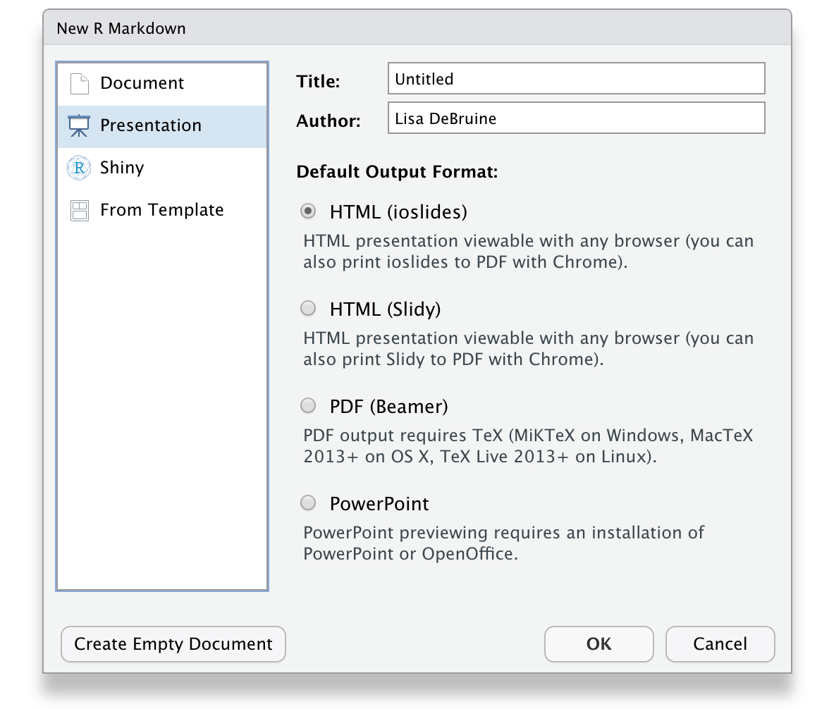
Figure 10.1: Ioslides RMarkdown template.
The main differences between this and the Rmd files you've been working with until now are that the output type in the YAML header is ioslides_presentation instead of html_document and this format requires a specific title structure. Each slide starts with a level-2 header.
The template provides you with examples of text, bullet point, code, and plot slides. You can knit this template to create an HTML document with your presentation. It often looks odd in the RStudio built-in browser, so click the button to open it in a web browser. You can use the space bar or arrow keys to advance slides.
The code below shows how to load some packages and display text, a table, and a plot. You can see the HTML output here.
---
title: "Presentation Demo"
author: "Lisa DeBruine"
output: ioslides_presentation
---

```{r setup, include=FALSE}
knitr::opts_chunk$set(echo = FALSE)
library(tidyverse)
library(kableExtra)
```

## Slide with Markdown

The following slides will present some data from the `diamonds` dataset from **ggplot2**.

Diamond price depends on many features, such as:

- cut
- colour
- clarity
- carats

## Slide with a Table

```{r}
diamonds %>%
  group_by(cut, color) %>%
  summarise(avg_price = mean(price),
            .groups = "drop") %>%
  pivot_wider(names_from = cut, values_from = avg_price) %>%
  kable(digits = 0, caption = "Mean diamond price by cut and colour.") %>%
  kable_material()
```

## Slide with a Plot

```{r pressure}
ggplot(diamonds, aes(x = cut, y = price, color = color)) +
  stat_summary(fun = mean, geom = "point") +
  stat_summary(aes(x = as.integer(cut)),
               fun = mean, geom = "line") +
  scale_x_discrete(position = "top") +
  scale_color_viridis_d(guide = guide_legend(reverse = TRUE)) +
  theme_minimal()
```
10.3.2 Dashboards
Dashboards are a way to display text, tables, and plots with dynamic formatting. After you install flexdashboard, you can choose a flexdashboard template when you create a new R Markdown document.
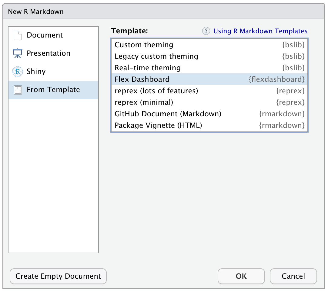
Figure 10.2: Flexdashboard RMarkdown template.
The code below shows how to load some packages, display two tables in a tabset, and display two plots in a column. You can see the HTML output here.
---
title: "Flexdashboard Demo"
output:
  flexdashboard::flex_dashboard:
    social: [ "twitter", "facebook", "linkedin", "pinterest" ]
    source_code: embed
    orientation: columns
    vertical_layout: fill
---

```{r setup, include=FALSE}
library(flexdashboard)
library(tidyverse)
library(kableExtra)
library(DT) # for interactive tables
theme_set(theme_minimal())
```

Column {data-width=350, .tabset}
--------------------------------

### By Cut

This table uses `kableExtra` to render the table with a specific theme.

```{r}
diamonds %>%
  group_by(cut) %>%
  summarise(avg = mean(price),
            .groups = "drop") %>%
  kable(digits = 0,
        col.names = c("Cut", "Average Price"),
        caption = "Mean diamond price by cut.") %>%
  kable_classic()
```

### By Colour

This table uses `DT::datatable()` to render the table with a searchable interface.

```{r}
diamonds %>%
  group_by(color) %>%
  summarise(avg = mean(price),
            .groups = "drop") %>%
  DT::datatable(colnames = c("Colour", "Average Price"),
                caption = "Mean diamond price by colour",
                options = list(pageLength = 5),
                rownames = FALSE) %>%
  DT::formatRound(columns=2, digits=0)
```

Column {data-width=350}
-----------------------

### By Clarity

```{r by-clarity, fig.cap = "Diamond price by clarity"}
ggplot(diamonds, aes(x = clarity, y = price)) +
  geom_boxplot()
```


### By Carats

```{r by-carat, fig.cap = "Diamond price by carat"}
ggplot(diamonds, aes(x = carat, y = price)) +
  stat_smooth()
```
Change the size of your web browser to see how the boxes, tables and figures change.
The best way to figure out how to format a dashboard is trial and error, but you can also look at some sample layouts.
10.3.3 Books
You can create online books with bookdown. In fact, the book you're reading was created using bookdown. After you download the package, start a new project and choose "Book project using bookdown" from the list of project templates.
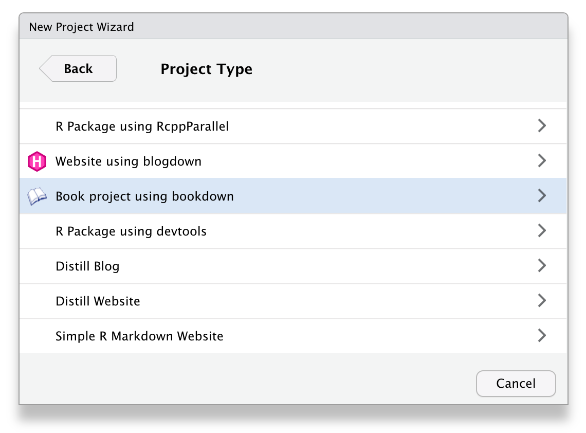
Figure 10.3: Bookdown project template.
Each chapter is written in a separate .Rmd file and the general book settings can be changed in the _bookdown.yml and _output.yml files.
10.3.4 Websites
You can create a simple website the same way you create any R Markdown document. Choose "Simple R Markdown Website" from the project templates to get started. See Appendix L for a step-by-step tutorial.
For more complex, blog-style websites, you can investigate blogdown. After you install this package, you will also be able to crate template blogdown projects to get you started.
10.3.5 Shiny
To get truly interactive, you can take your R coding to the next level and learn Shiny. Shiny apps let your R code react to user input. You can do things like make a word cloud, search a google spreadsheet, or conduct a survey.
This is well outside the scope of this class, but the skills you've learned here provide a good start. The free book Building Web Apps with R Shiny by one of the authors of this book can get you started creating shiny apps.