F Data Types
F.1 Basic data types
Data can be numbers, words, true/false values or combinations of these. The basic data types in R are: numeric, character, and logical, as well as the special classes of factor and date/times.
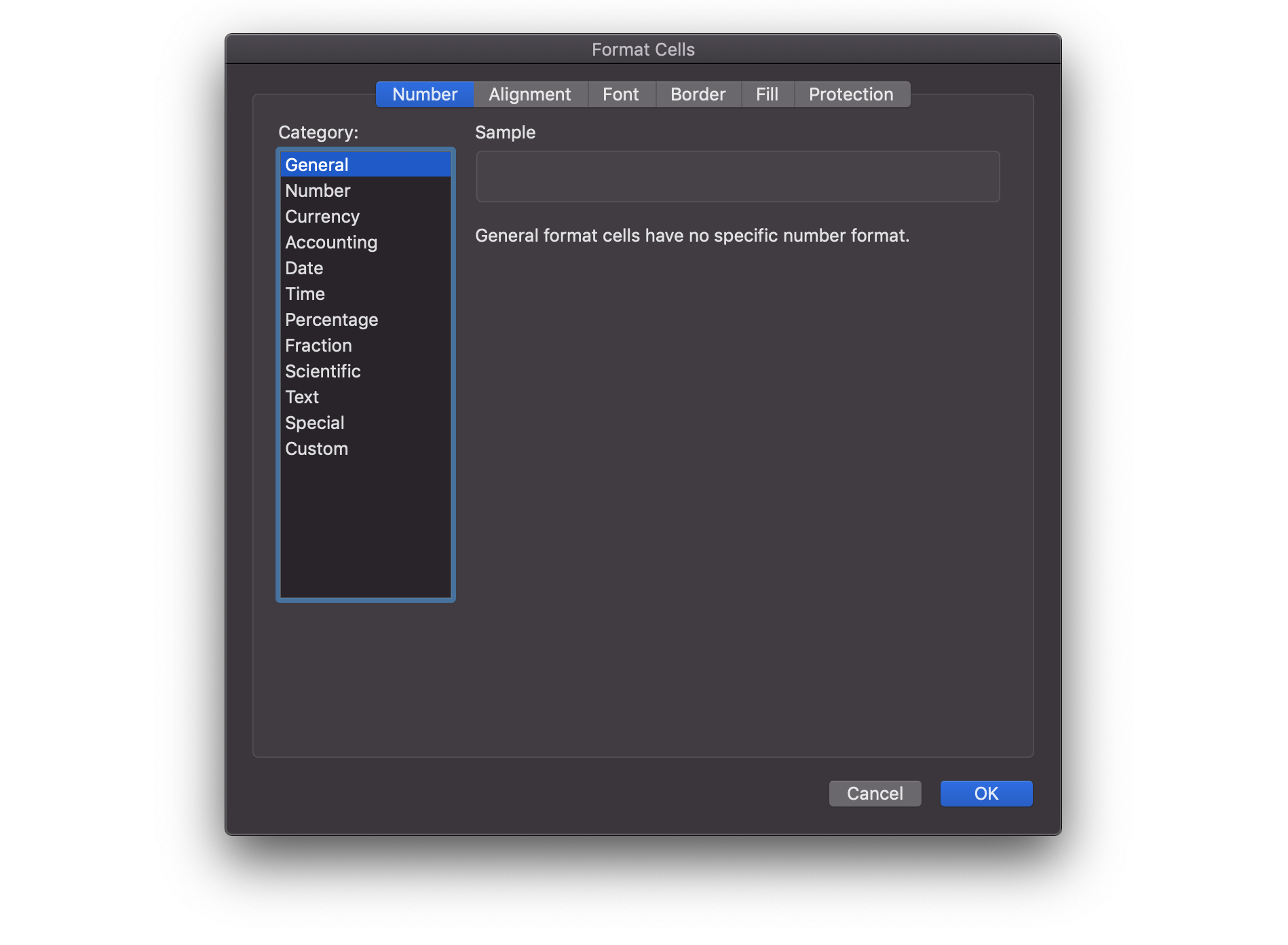
Figure F.1: Data types are like the categories when you format cells in Excel.
F.1.1 Numeric data
All of the numbers are numeric data types. There are two types of numeric data, integer and double. Integers are the whole numbers, like -1, 0 and 1. Doubles are numbers that can have fractional amounts. If you just type a plain number such as 10, it is stored as a double, even if it doesn't have a decimal point. If you want it to be an exact integer, you can use the L suffix (10L), but this distinction doesn't make much difference in practice.
If you ever want to know the data type of something, use the typeof function.
## [1] "double"
## [1] "double"
## [1] "integer"
If you want to know if something is numeric (a double or an integer), you can use the function is.numeric() and it will tell you if it is numeric (TRUE) or not (FALSE).
is.numeric(10L)
is.numeric(10.0)
is.numeric("Not a number")
## [1] TRUE
## [1] TRUE
## [1] FALSEF.1.2 Character data
Characters (also called "strings") are any text between quotation marks.
## [1] "character"
## [1] "character"
This can include quotes, but you have to escape quotes using a backslash to signal that the quote isn't meant to be the end of the string.
my_string <- "The instructor said, \"R is cool,\" and the class agreed."
cat(my_string) # cat() prints the arguments
## The instructor said, "R is cool," and the class agreed.F.1.3 Logical Data
Logical data (also sometimes called "boolean" values) is one of two values: true or false. In R, we always write them in uppercase: TRUE and FALSE.
## [1] "logical"
## [1] "logical"
When you compare two values with an operator, such as checking to see if 10 is greater than 5, the resulting value is logical.
is.logical(10 > 5)## [1] TRUEYou might also see logical values abbreviated as T and F, or 0 and 1. This can cause some problems down the road, so we will always spell out the whole thing.
F.1.4 Factors
A factor is a specific type of integer that lets you specify the categories and their order. This is useful in data tables to make plots display with categories in the correct order.
## [1] B
## Levels: A B C
Factors are a type of integer, but you can tell that they are factors by checking their class().
## [1] "integer"
## [1] "factor"
F.1.5 Dates and Times
Dates and times are represented by doubles with special classes. Although typeof() will tell you they are a double, you can tell that they are dates by checking their class(). Datetimes can have one or more of a few classes that start with POSIX.
date <- as.Date("2022-01-24")
datetime <- ISOdatetime(2022, 1, 24, 10, 35, 00, "GMT")
typeof(date)
typeof(datetime)
class(date)
class(datetime)
## [1] "double"
## [1] "double"
## [1] "Date"
## [1] "POSIXct" "POSIXt"See Appendix G for how to use lubridate to work with dates and times.
What data types are these:
-
100 -
100L -
"100" -
100.0 -
-100L -
factor(100) -
TRUE -
"TRUE" -
FALSE -
1 == 2
F.2 Basic container types
Individual data values can be grouped together into containers. The main types of containers we'll work with are vectors, lists, and data tables.
F.2.1 Vectors
A vector in R is a set of items (or 'elements') in a specific order. All of the elements in a vector must be of the same data type (numeric, character, logical). You can create a vector by enclosing the elements in the function c().
## put information into a vector using c(...)
c(1, 2, 3, 4)
c("this", "is", "cool")
1:6 # shortcut to make a vector of all integers x:y
## [1] 1 2 3 4
## [1] "this" "is" "cool"
## [1] 1 2 3 4 5 6What happens when you mix types? What class is the variable mixed?
mixed <- c(2, "good", 2L, "b", TRUE)
typeof(mixed)## [1] "character"You can't mix data types in a vector; all elements of the vector must be the same data type. If you mix them, R will coerce them so that they are all the same. If you mix doubles and integers, the integers will be changed to doubles. If you mix characters and numeric types, the numbers will be coerced to characters, so 10 would turn into "10".
F.2.1.1 Selecting values from a vector
If we wanted to pick specific values out of a vector by position, we can use square brackets (an extract operator, or []) after the vector.
values <- c(10, 20, 30, 40, 50)
values[2] # selects the second value
## [1] 20You can select more than one value from the vector by putting a vector of numbers inside the square brackets. For example, you can select the 18th, 19th, 20th, 21st, 4th, 9th and 15th letter from the built-in vector LETTERS (which gives all the uppercase letters in the Latin alphabet).
word <- c(18, 19, 20, 21, 4, 9, 15)
LETTERS[word]
## [1] "R" "S" "T" "U" "D" "I" "O"Can you decode the secret message?
secret <- c(14, 5, 22, 5, 18, 7, 15, 14, 14, 1, 7, 9, 22, 5, 25, 15, 21, 21, 16)
LETTERS[secret]## [1] "N" "E" "V" "E" "R" "G" "O" "N" "N" "A" "G" "I" "V" "E" "Y" "O" "U" "U" "P"You can also create 'named' vectors, where each element has a name. For example:
vec <- c(first = 77.9, second = -13.2, third = 100.1)
vec
## first second third
## 77.9 -13.2 100.1We can then access elements by name using a character vector within the square brackets. We can put them in any order we want, and we can repeat elements:
vec[c("third", "second", "second")]## third second second
## 100.1 -13.2 -13.2We can get the vector of names using the names() function, and we can set or change them using something like names(vec2) <- c("n1", "n2", "n3").
Another way to access elements is by using a logical vector within the square brackets. This will pull out the elements of the vector for which the corresponding element of the logical vector is TRUE. If the logical vector doesn't have the same length as the original, it will repeat. You can find out how long a vector is using the length() function.
## [1] 26
##  [1] "A" "C" "E" "G" "I" "K" "M" "O" "Q" "S" "U" "W" "Y"
F.2.1.2 Repeating Sequences
Here are some useful tricks to save typing when creating vectors.
In the command x:y the : operator would give you the sequence of number starting at x, and going to y in increments of 1.
1:10
15.3:20.5
0:-10
## [1] 1 2 3 4 5 6 7 8 9 10
## [1] 15.3 16.3 17.3 18.3 19.3 20.3
## [1] 0 -1 -2 -3 -4 -5 -6 -7 -8 -9 -10What if you want to create a sequence but with something other than integer steps? You can use the seq() function. Look at the examples below and work out what the arguments do.
##  [1] -1.0 -0.8 -0.6 -0.4 -0.2  0.0  0.2  0.4  0.6  0.8  1.0
##  [1]   0  10  20  30  40  50  60  70  80  90 100
##  [1]  0.0  0.4  0.8  1.2  1.6  2.0  2.4  2.8  3.2  3.6  4.0  4.4  4.8  5.2  5.6
## [16]  6.0  6.4  6.8  7.2  7.6  8.0  8.4  8.8  9.2  9.6 10.0
What if you want to repeat a vector many times? You could either type it out (painful) or use the rep() function, which can repeat vectors in different ways.
rep(0, 10)                      # ten zeroes
rep(c(1L, 3L), times = 7)       # alternating 1 and 3, 7 times
rep(c("A", "B", "C"), each = 2) # A to C, 2 times each
## [1] 0 0 0 0 0 0 0 0 0 0
## [1] 1 3 1 3 1 3 1 3 1 3 1 3 1 3
## [1] "A" "A" "B" "B" "C" "C"The rep() function is useful to create a vector of logical values (TRUE/FALSE or 1/0) to select values from another vector.
# Get IDs in the pattern Y Y N N ...
ids <- 1:40
yynn <- rep(c(TRUE, FALSE), each = 2,
            length.out = length(ids))
ids[yynn]
## [1] 1 2 5 6 9 10 13 14 17 18 21 22 25 26 29 30 33 34 37 38F.2.2 Lists
Recall that vectors can contain data of only one type. What if you want to store a collection of data of different data types? For that purpose you would use a list. Define a list using the list() function.
data_types <- list(
  double = 10.0,
  integer = 10L,
  character = "10",
  logical = TRUE
)

str(data_types) # str() prints lists in a condensed format
## List of 4
## $ double : num 10
## $ integer : int 10
## $ character: chr "10"
## $ logical : logi TRUEYou can refer to elements of a list using square brackets like a vector, but you can also use the dollar sign notation ($) if the list items have names.
data_types$logical## [1] TRUEExplore the 5 ways shown below to extract a value from a list. What data type is each object? What is the difference between the single and double brackets? Which one is the same as the dollar sign?
bracket1 <- data_types[1]
bracket2 <- data_types[[1]]
name1    <- data_types["double"]
name2    <- data_types[["double"]]
dollar   <- data_types$double
The single brackets (bracket1 and name1) return a list with the subset of items inside the brackets. In this case, that's just one item, but can be more (try data_types[1:2]). The items keep their names if they have them, so the returned value is list(double = 10).
The double brackets (bracket2 and name2 return a single item as a vector. You can't select more than one item; data_types[[1:2]] will give you a "subscript out of bounds" error.
The dollar-sign notation is the same as double-brackets. If the name has spaces or any characters other than letters, numbers, underscores, and full stops, you need to surround the name with backticks (e.g., sales$`Customer ID`).
F.2.3 Tables
Tabular data structures allow for a collection of data of different types (characters, integers, logical, etc.) but subject to the constraint that each "column" of the table (element of the list) must have the same number of elements. The base R version of a table is called a data.frame, while the 'tidyverse' version is called a tibble. Tibbles are far easier to work with, so we'll be using those. To learn more about differences between these two data structures, see vignette("tibble").
# construct a table by column with tibble
avatar <- tibble(
  name = c("Katara", "Toph", "Sokka"),
  bends = c("water", "earth", NA),
  friendly = TRUE
)

# or by row with tribble
avatar <- tribble(
  ~name,    ~bends,  ~friendly,
  "Katara", "water", TRUE,
  "Toph",   "earth", TRUE,
  "Sokka",  NA,      TRUE
)
# export the data to a file
rio::export(avatar, "data/avatar.csv")

# or by importing data from a file
avatar <- rio::import("data/avatar.csv")
Tabular data becomes especially important for when we talk about tidy data in Chapter 8, which consists of a set of simple principles for structuring data.
F.2.3.1 Table info
We can get information about the table using the following functions.
-
ncol(): number of columns -
nrow(): number of rows -
dim(): the number of rows and number of columns -
name(): the column names -
glimpse(): the column types
## [1] 3
## [1] 3
## [1] 3 3
## [1] "name"     "bends"    "friendly"
## Rows: 3
## Columns: 3
## $ name     <chr> "Katara", "Toph", "Sokka"
## $ bends    <chr> "water", "earth", NA
## $ friendly <lgl> TRUE, TRUE, TRUE
F.2.3.2 Accessing rows and columns
There are various ways of accessing specific columns or rows from a table. You'll be learning more about this in Chapters 8 and 9.
siblings   <- avatar %>% slice(1, 3) # rows (by number)
bends      <- avatar %>% pull(2) # column vector (by number)
friendly   <- avatar %>% pull(friendly) # column vector (by name)
bends_name <- avatar %>% select(bends, name) # subset table (by name)
toph       <- avatar %>% pull(name) %>% pluck(2) # single cell
The code below uses base R to produce the same subsets as the functions above. This format is useful to know about, since you might see them in other people's scripts.
F.3 Glossary
| term | definition |
|---|---|
| base r | The set of R functions that come with a basic installation of R, before you add external packages |
| character | A data type representing strings of text. |
| coercion | Changing the data type of values in a vector to a single compatible type. |
| data type | The kind of data represented by an object. |
| double | A data type representing a real decimal number |
| escape | Include special characters like " inside of a string by prefacing them with a backslash. |
| extract operator | A symbol used to get values from a container object, such as [, [[, or $ |
| factor | A data type where a specific set of values are stored with labels; An explanatory variable manipulated by the experimenter |
| integer | A data type representing whole numbers. |
| list | A container data type that allows items with different data types to be grouped together. |
| logical | A data type representing TRUE or FALSE values. |
| numeric | A data type representing a real decimal number or integer. |
| operator | A symbol that performs a mathematical operation, such as +, -, *, / |
| tabular data | Data in a rectangular table format, where each row has an entry for each column. |
| tidy data | A format for data that maps the meaning onto the structure. |
| vector | A type of data structure that collects values with the same data type, like T/F values, numbers, or strings. |