7 Data Relations

7.1 Intended Learning Outcomes

• Be able to match related data across multiple tables
• Be able to combine data from multiple files

7.2 Walkthrough video

There is a walkthrough video of this chapter available via Echo360. Please note that there may have been minor edits to the book since the video was recorded. Where there are differences, the book should always take precedence.

7.3 Set-up

First, create a new project for the work we'll do in this chapter named 07-relations. Second, open and save a new R Markdown document named relations.Rmd, delete the welcome text, and load the required packages for this chapter.

```{r setup, include=FALSE}

library(tidyverse)     # includes readr & tibble

```

Download the Data transformation cheatsheet.

7.4 Loading data

The data you want to report on or visualise are often in more than one file (or more than one tab of an excel file or googlesheet). You might need to join up a table of customer information with a table of orders, or combine the monthly social media reports across several months.

For this demo, rather than loading in data, we'll create two small data tables from scratch using the tibble() function.

customers has id, city and postcode for five customers 1-5.

• 1:5 will fill the variable id with all integers between 1 and 5.
• city and code both use the c() function to enter multiple strings. Note that each entry is contained within its own quotation marks, apart from missing data, which is recorded as NA.
• When entering data like this, it's important that the order of each variable matches up. So number 1 will correspond to "Port Ellen" and "PA42 7DU".

customers <- tibble(
  id = 1:5,
  city = c("Port Ellen", "Dufftown", NA, "Aberlour", "Tobermory"),
  postcode = c("PA42 7DU", "AB55 4DH", NA, "AB38 7RY", "PA75 6NR")
)

Table 7.1: Demo customers table.

id	city	postcode
1	Port Ellen	PA42 7DU
2	Dufftown	AB55 4DH
3	NA	NA
4	Aberlour	AB38 7RY
5	Tobermory	PA75 6NR

orders has customer id and the number of items ordered. Some customers from the previous table have no orders, some have more than one order, and some are not in the customer table.

orders <- tibble(
  id = c(2, 3, 4, 4, 5, 5, 6, 6, 7),
  items = c(10, 18, 21, 23, 9, 11, 11, 12, 3)
)

Table 7.2: Demo orders table.

id	items
2	10
3	18
4	21
4	23
5	9
5	11
6	11
6	12
7	3

7.5 Mutating Joins

Mutating joins act like the dplyr::mutate() function in that they add new columns to one table based on values in another table. (We'll learn more about the mutate() function in Chapter 8.)

All the mutating joins have this basic syntax:

****_join(x, y, by = NULL, suffix = c(".x", ".y"))

• x = the first (left) table
• y = the second (right) table
• by = what columns to match on. If you leave this blank, it will match on all columns with the same names in the two tables.
• suffix = if columns have the same name in the two tables, but you aren't joining by them, they get a suffix to make them unambiguous. This defaults to ".x" and ".y", but you can change it to something more meaningful.

You can leave out the by argument if you're matching on all of the columns with the same name, but it's good practice to always specify it so your code is robust to changes in the loaded data.

7.5.1 left_join()

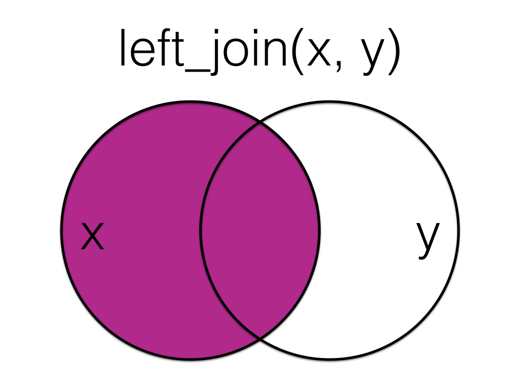
A left_join keeps all the data from the first (left) table and adds anything that matches from the second (right) table. If the right table has more than one match for a row in the left table, there will be more than one row in the joined table (see ids 4 and 5).

left_data <- left_join(customers, orders, by = "id")
left_data

id	city	postcode	items
1	Port Ellen	PA42 7DU	NA
2	Dufftown	AB55 4DH	10
3	NA	NA	18
4	Aberlour	AB38 7RY	21
4	Aberlour	AB38 7RY	23
5	Tobermory	PA75 6NR	9
5	Tobermory	PA75 6NR	11

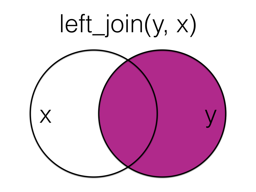
The order you specify the tables matters, in the below code we have reversed the order and so the result is all rows from the orders table joined to any matching rows from the customers table.

left2_data <- left_join(orders, customers, by = "id")
left2_data

id	items	city	postcode
2	10	Dufftown	AB55 4DH
3	18	NA	NA
4	21	Aberlour	AB38 7RY
4	23	Aberlour	AB38 7RY
5	9	Tobermory	PA75 6NR
5	11	Tobermory	PA75 6NR
6	11	NA	NA
6	12	NA	NA
7	3	NA	NA

7.5.2 right_join()

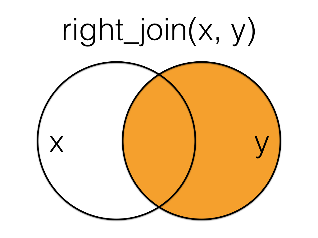
A right_join keeps all the data from the second (right) table and joins anything that matches from the first (left) table.

right_data <- right_join(customers, orders, by = "id")
right_data

id	city	postcode	items
2	Dufftown	AB55 4DH	10
3	NA	NA	18
4	Aberlour	AB38 7RY	21
4	Aberlour	AB38 7RY	23
5	Tobermory	PA75 6NR	9
5	Tobermory	PA75 6NR	11
6	NA	NA	11
6	NA	NA	12
7	NA	NA	3

This table has the same information as left_join(orders, customers, by = "id"), but the columns are in a different order (left table, then right table).

7.5.3 inner_join()

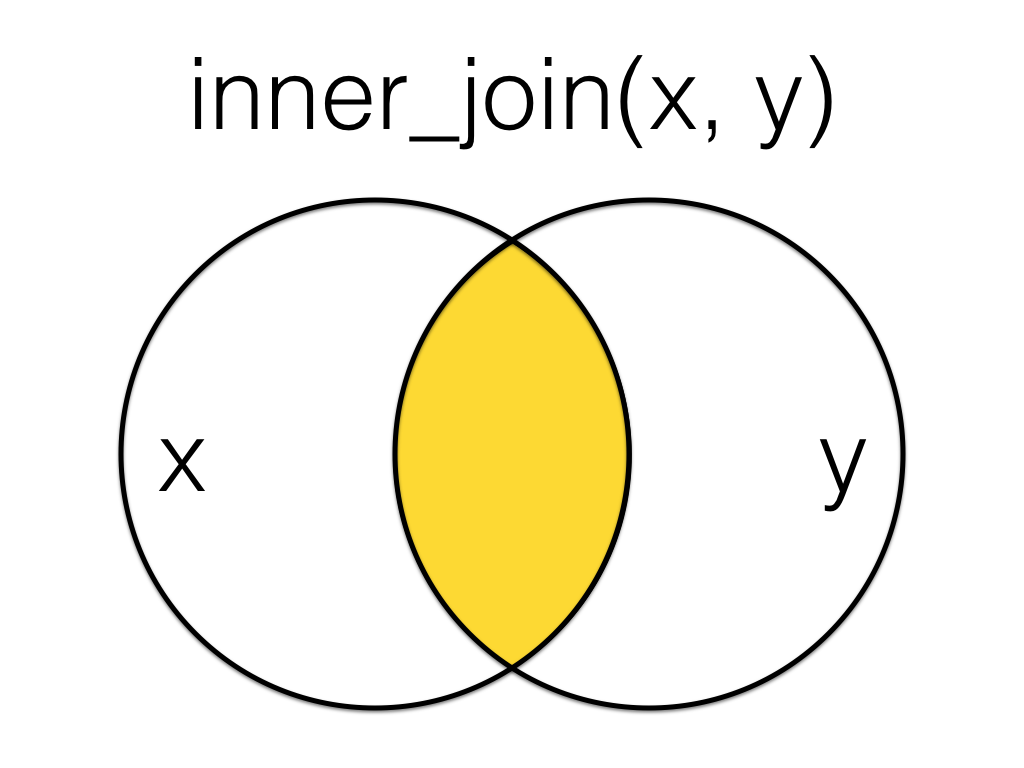
An inner_join returns all the rows that have a match in both tables. Changing the order of the tables will change the order of the columns, but not which rows are kept.

inner_data <- inner_join(customers, orders, by = "id")
inner_data

id	city	postcode	items
2	Dufftown	AB55 4DH	10
3	NA	NA	18
4	Aberlour	AB38 7RY	21
4	Aberlour	AB38 7RY	23
5	Tobermory	PA75 6NR	9
5	Tobermory	PA75 6NR	11

7.5.4 full_join()

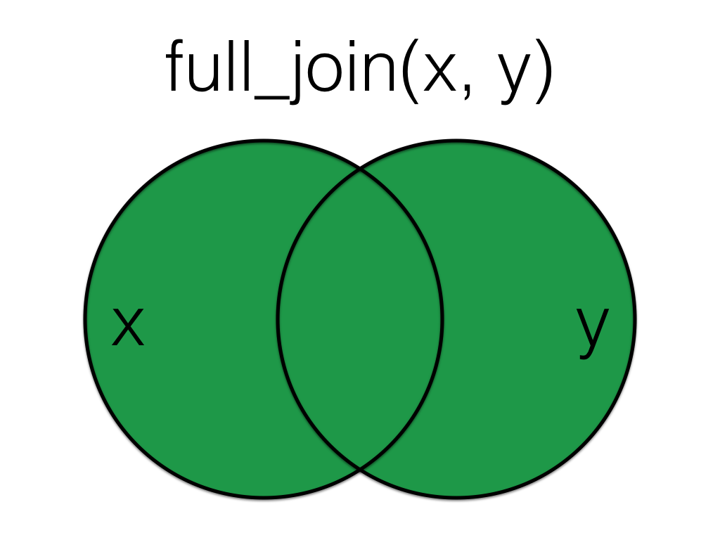
A full_join lets you join up rows in two tables while keeping all of the information from both tables. If a row doesn't have a match in the other table, the other table's column values are set to NA.

full_data <- full_join(customers, orders, by = "id")
full_data

id	city	postcode	items
1	Port Ellen	PA42 7DU	NA
2	Dufftown	AB55 4DH	10
3	NA	NA	18
4	Aberlour	AB38 7RY	21
4	Aberlour	AB38 7RY	23
5	Tobermory	PA75 6NR	9
5	Tobermory	PA75 6NR	11
6	NA	NA	11
6	NA	NA	12
7	NA	NA	3

7.6 Filtering Joins

Filtering joins act like the dplyr::filter() function in that they keep and remove rows from the data in one table based on the values in another table. The result of a filtering join will only contain rows from the left table and have the same number or fewer rows than the left table. (We'll learn more about the filter() function in Chapter 9.)

7.6.1 semi_join()

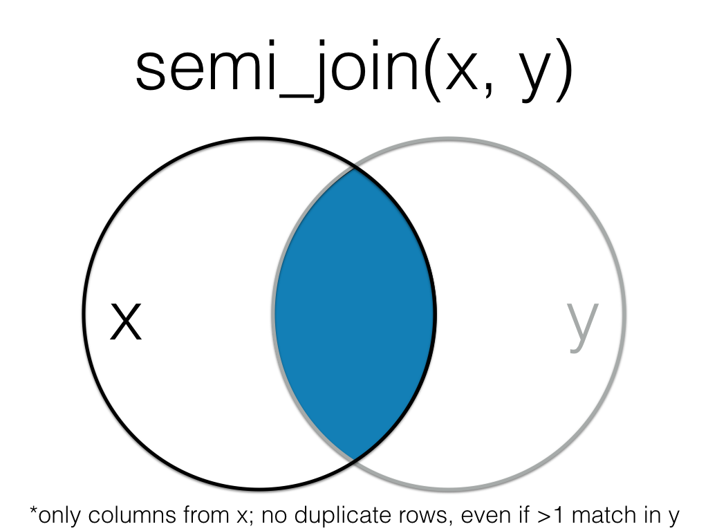
A semi_join returns all rows from the left table where there are matching values in the right table, keeping just columns from the left table.

semi_data <- semi_join(customers, orders, by = "id")
semi_data

id	city	postcode
2	Dufftown	AB55 4DH
3	NA	NA
4	Aberlour	AB38 7RY
5	Tobermory	PA75 6NR

Unlike an inner join, a semi join will never duplicate the rows in the left table if there is more than one matching row in the right table.

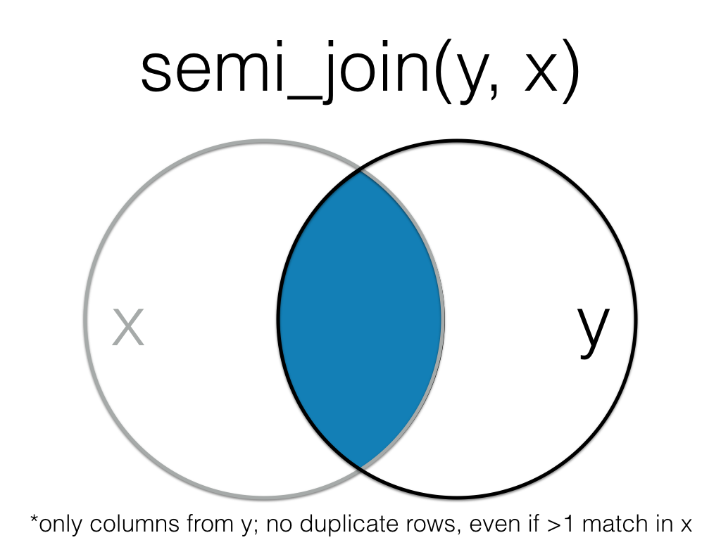
Order matters in a semi join.

semi2_data <- semi_join(orders, customers, by = "id")
semi2_data

id	items
2	10
3	18
4	21
4	23
5	9
5	11

7.6.2 anti_join()

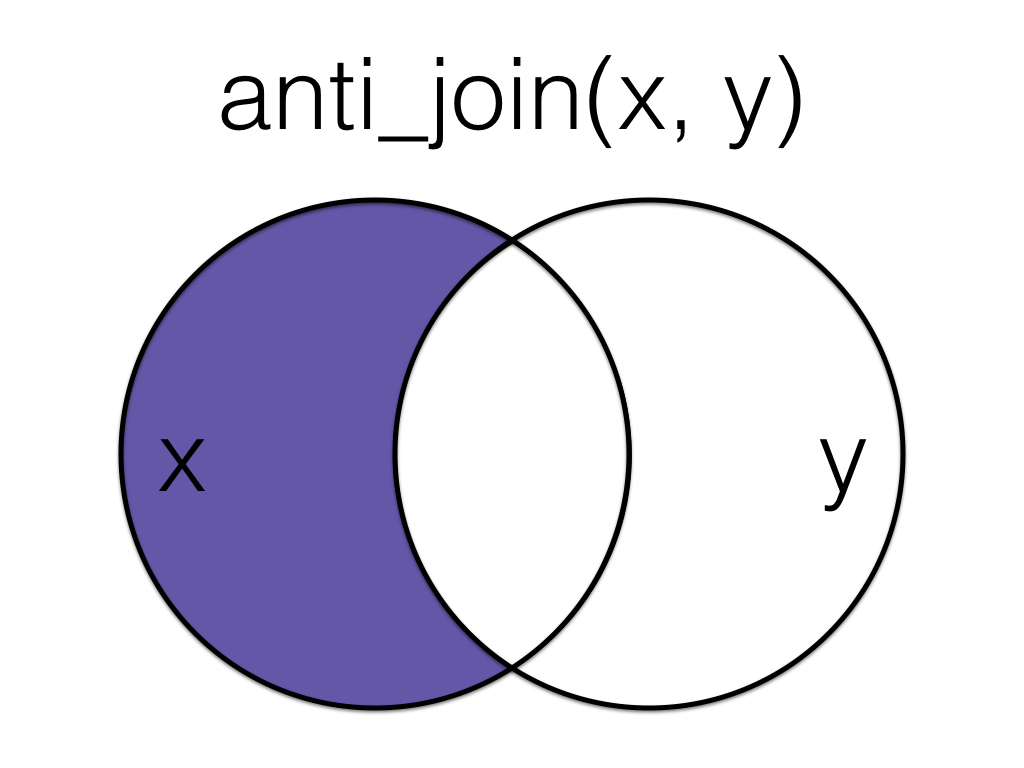
An anti_join return all rows from the left table where there are not matching values in the right table, keeping just columns from the left table.

anti_data <- anti_join(customers, orders, by = "id")
anti_data

id	city	postcode
1	Port Ellen	PA42 7DU

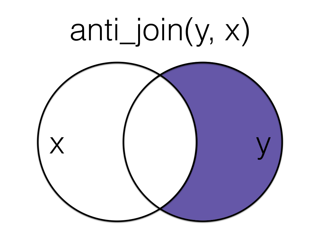
Order matters in an anti join.

anti2_data <- anti_join(orders, customers, by = "id")
anti2_data

id	items
6	11
6	12
7	3

7.7 Multiple joins

The ****_join() functions are all two-table verbs, that is, you can only join together two tables at a time. However, you may often need to join together multiple tables. To do so, you simply need to add on additional joins. You can do this by creating an intermediate object or more efficiently by using a pipe.

# create a table of overall customer satisfaction scores
satisfaction <- tibble(
  id = 1:5,
  satisfaction = c(4, 3, 2, 3, 1)
)

# perform the initial join
join_1 <- left_join(customers, orders, by = "id")

# perform the second join on the new object
join_2 <- left_join(join_1, satisfaction, 
                    by = "id")

# more efficient method using the pipe
pipe_join <- customers %>%
  left_join(orders, by = "id") %>%
  left_join(satisfaction, by = "id")

At every stage of any analysis you should check your output to ensure that what you created is what you intended to create, but this is particularly true of joins. You should be familiar enough with your data through routine checks using functions like glimpse(), str(), and summary() to have a rough idea of what the join should result in. At the very least, you should know whether the joined object should result in more or fewer variables and observations.

If you have a multi-line join like in the above piped example, build up the code and check the output at each stage.

7.8 Binding Joins

Binding joins bind one table to another by adding their rows or columns together.

7.8.1 bind_rows()

You can combine the rows of two tables with bind_rows.

Here we'll add customer data for customers 6-9 and bind that to the original customer table.

new_customers <- tibble(
  id = 6:9,
  city = c("Falkirk", "Ardbeg", "Doogal", "Kirkwall"),
  postcode = c("FK1 4RS", "PA42 7EA", "G81 4SJ", "KW15 1SE")
)

bindr_data <- bind_rows(customers, new_customers)
bindr_data

id	city	postcode
1	Port Ellen	PA42 7DU
2	Dufftown	AB55 4DH
3	NA	NA
4	Aberlour	AB38 7RY
5	Tobermory	PA75 6NR
6	Falkirk	FK1 4RS
7	Ardbeg	PA42 7EA
8	Doogal	G81 4SJ
9	Kirkwall	KW15 1SE

The columns just have to have the same names, they don't have to be in the same order. Any columns that differ between the two tables will just have NA values for entries from the other table.

If a row is duplicated between the two tables (like id 5 below), the row will also be duplicated in the resulting table. If your tables have the exact same columns, you can use union() (see Section 7.9.2) to avoid duplicates.

new_customers <- tibble(
  id = 5:9,
  postcode = c("PA75 6NR", "FK1 4RS", "PA42 7EA", "G81 4SJ", "KW15 1SE"),
  city = c("Tobermory", "Falkirk", "Ardbeg", "Doogal", "Kirkwall"),
  new = c(1,2,3,4,5)
)

bindr2_data <- bind_rows(customers, new_customers)
bindr2_data

id	city	postcode	new
1	Port Ellen	PA42 7DU	NA
2	Dufftown	AB55 4DH	NA
3	NA	NA	NA
4	Aberlour	AB38 7RY	NA
5	Tobermory	PA75 6NR	NA
5	Tobermory	PA75 6NR	1
6	Falkirk	FK1 4RS	2
7	Ardbeg	PA42 7EA	3
8	Doogal	G81 4SJ	4
9	Kirkwall	KW15 1SE	5

7.8.2 bind_cols()

You can merge two tables with the same number of rows using bind_cols. This is only useful if the two tables have the same number of rows in the exact same order.

new_info <- tibble(
  colour = c("red", "orange", "yellow", "green", "blue")
)

bindc_data <- bind_cols(customers, new_info)
bindc_data 

id	city	postcode	colour
1	Port Ellen	PA42 7DU	red
2	Dufftown	AB55 4DH	orange
3	NA	NA	yellow
4	Aberlour	AB38 7RY	green
5	Tobermory	PA75 6NR	blue

The only advantage of bind_cols() over a mutating join is when the tables don't have any IDs to join by and you have to rely solely on their order. Otherwise, you should use a mutating join (all four mutating joins result in the same output when all rows in each table have exactly one match in the other table).

7.8.3 Importing multiple files

If you need to import and bind a whole folder full of files that have the same structure, get a list of all the files you want to combine. It's easiest if they're all in the same directory, although you can use a pattern to select the files you want if they have a systematic naming structure.

First, save the two customer tables to CSV files. The dir.create() function makes a folder called "data". The showWarnings = FALSE argument means that you won't get a warning if the folder already exists, it just won't do anything.

# write our data to a new folder for the demo
dir.create("data", showWarnings = FALSE)
write_csv(x = customers, file = "data/customers1.csv")
write_csv(x = new_customers, file = "data/customers2.csv")

Next, retrieve a list of all file names in the data folder that contain the string "customers"

files <- list.files(
  path = "data", 
  pattern = "customers", 
  full.names = TRUE
)

files

## [1] "data/customers1.csv" "data/customers2.csv"

Next, we'll iterate over this list to read in the data from each file. Whilst this won't be something we cover in detail in the core resources of this course, iteration is an important concept to know about. Iteration is where you perform the same task on multiple different inputs. As a general rule of thumb, if you find yourself copying and pasting the same thing more than twice, there's a more efficient and less error-prone way to do it, although these functions do typically require a stronger grasp of programming.

The purrr package contains functions to help with iteration. purrr::map_df() maps a function to a list and returns a data frame (table) of the results.

• .x is the list of file paths
• .f specifies the function to map to each of those file paths.
• The resulting object all_files will be a data frame that combines all the files together, similar to if you had imported them separately and then used bind_rows(). Note that map_df() will only work in this way if the structure of all files is identical.

all_files <- purrr::map_df(.x = files, .f = read_csv)

7.9 Set Operations

Set operations compare two tables and return rows that match (intersect), are in either table (union), or are in one table but not the other (setdiff).

7.9.1 intersect()

dplyr::intersect() returns all rows in two tables that match exactly. The columns don't have to be in the same order, but they have to have the same names.

new_customers <- tibble(
  id = 5:9,
  postcode = c("PA75 6NR", "FK1 4RS", "PA42 7EA", "G81 4SJ", "KW15 1SE"),
  city = c("Tobermory", "Falkirk", "Ardbeg", "Doogal", "Kirkwall")
)

intersect_data <- intersect(customers, new_customers)
intersect_data

id	city	postcode
5	Tobermory	PA75 6NR

If you've forgotten to load dplyr or the tidyverse, base R also has a base::intersect() function that doesn't work like dplyr::intersect(). The error message can be confusing and looks something like this:

base::intersect(customers, new_customers)

## Error in `vectbl_as_row_location()`:
## ! Must subset rows with a valid subscript vector.
## ℹ Logical subscripts must match the size of the indexed input.
## x Input has size 5 but subscript `!duplicated(x, fromLast = fromLast, ...)` has size 0.

7.9.2 union()

dplyr::union() returns all the rows from both tables, removing duplicate rows, unlike bind_rows().

union_data <- union(customers, new_customers)
union_data

id	city	postcode
1	Port Ellen	PA42 7DU
2	Dufftown	AB55 4DH
3	NA	NA
4	Aberlour	AB38 7RY
5	Tobermory	PA75 6NR
6	Falkirk	FK1 4RS
7	Ardbeg	PA42 7EA
8	Doogal	G81 4SJ
9	Kirkwall	KW15 1SE

If you've forgotten to load dplyr or the tidyverse, base R also has a base::union() function. You usually won't get an error message, but the output won't be what you expect.

base::union(customers, new_customers)

## [[1]]
## [1] 1 2 3 4 5
## 
## [[2]]
## [1] "Port Ellen" "Dufftown"   NA           "Aberlour"   "Tobermory" 
## 
## [[3]]
## [1] "PA42 7DU" "AB55 4DH" NA         "AB38 7RY" "PA75 6NR"
## 
## [[4]]
## [1] 5 6 7 8 9
## 
## [[5]]
## [1] "PA75 6NR" "FK1 4RS"  "PA42 7EA" "G81 4SJ"  "KW15 1SE"
## 
## [[6]]
## [1] "Tobermory" "Falkirk"   "Ardbeg"    "Doogal"    "Kirkwall"

7.9.3 setdiff()

dplyr::setdiff returns rows that are in the first table, but not in the second table.

setdiff_data <- setdiff(customers, new_customers)
setdiff_data

id	city	postcode
1	Port Ellen	PA42 7DU
2	Dufftown	AB55 4DH
3	NA	NA
4	Aberlour	AB38 7RY

Order matters for setdiff.

setdiff2_data <- setdiff(new_customers, customers)
setdiff2_data

id	postcode	city
6	FK1 4RS	Falkirk
7	PA42 7EA	Ardbeg
8	G81 4SJ	Doogal
9	KW15 1SE	Kirkwall

If you've forgotten to load dplyr or the tidyverse, base R also has a base::setdiff() function. You usually won't get an error message, but the output might not be what you expect because base::setdiff() expects columns to be in the same order, so id 5 here registers as different between the two tables.

base::setdiff(customers, new_customers)

id	city	postcode
1	Port Ellen	PA42 7DU
2	Dufftown	AB55 4DH
3	NA	NA
4	Aberlour	AB38 7RY
5	Tobermory	PA75 6NR

7.10 Conflicting variable types

As we covered in Chapter 4, when you import or create data, R will do its best to set each column to an appropriate data type. However, sometimes it gets it wrong or sometimes there's something in the way the data has been encoded in the original spreadsheet that causes the data type to be different than expected. When joining datasets by common columns, it's important that not only are the variable names identical, but the data type of those variables is identical.

Let's recreate our new_customers dataset but this time, we'll specify that id is a character variable.

new_customers2 <- tibble(
  id = as.character(5:9),
  postcode = c("PA75 6NR", "FK1 4RS", "PA42 7EA", "G81 4SJ", "KW15 1SE"),
  city = c("Tobermory", "Falkirk", "Ardbeg", "Doogal", "Kirkwall")
)
str(new_customers2)

## tibble [5 × 3] (S3: tbl_df/tbl/data.frame)
##  $ id      : chr [1:5] "5" "6" "7" "8" ...
##  $ postcode: chr [1:5] "PA75 6NR" "FK1 4RS" "PA42 7EA" "G81 4SJ" ...
##  $ city    : chr [1:5] "Tobermory" "Falkirk" "Ardbeg" "Doogal" ...

If you try to join this dataset to any of the other datasets where id is stored as a numeric variable, it will produce an error.

inner_join(customers, new_customers2)

## Joining, by = c("id", "city", "postcode")

## Error in `inner_join()`:
## ! Can't join on `x$id` x `y$id` because of incompatible types.
## ℹ `x$id` is of type <integer>>.
## ℹ `y$id` is of type <character>>.

The same goes for bind_rows():

bind_rows(customers, new_customers2)

## Error in `bind_rows()`:
## ! Can't combine `..1$id` <integer> and `..2$id` <character>.

As alternative method to change variable types from what we showed you in Chapter 4 is to use the as.*** functions. If you type as. into a code chunk, you will see that there are a huge number of these functions for transforming variables and datasets to different types. Exactly which one you need will depend on the data you have, but a few commonly used ones are:

• as.numeric() - convert a variable to numeric. Useful for when you have a variable of real numbers that have been encoded as character. Any values that can't be turned into numbers (e.g., if you have the word "missing" in cells that you have no data for), will be returned as NA.
• as.factor() - convert a variable to a factor. You can set the factor levels and labels manually, or use the default order (alphabetical).
• as.character() - convert a variable to character data.
• as.tibble() and as.data.frame() - convert a list object (not a variable) to a tibble or a data frame (two different table formats). This isn't actually relevant to what we're discussing here, but it's a useful one to be aware of because sometimes you'll run into issues where you get an error that specifically requests your data is a tibble or data frame type and you can use this function to overwrite your object.

To use these functions on a variable we can use mutate() to overwrite the variable with that variable as the new data type:

new_customers2 <- new_customers2 %>%
  mutate(id = as.numeric(id))

Once you've done this, the joins will now work:

inner_join(orders, new_customers2)

## Joining, by = "id"

id	items	postcode	city
5	9	PA75 6NR	Tobermory
5	11	PA75 6NR	Tobermory
6	11	FK1 4RS	Falkirk
6	12	FK1 4RS	Falkirk
7	3	PA42 7EA	Ardbeg

7.11 Exercises

There's lots of different use cases for the ****_join() functions. These exercises will allow you to practice different joins. If you have any examples of where joins might be helpful in your own work, please post them on Teams in the week 6 channel, as having many concrete examples can help distinguish between the different joins.

7.11.1 Grade data

The University of Glasgow's Schedule A grading scheme uses a 22-point alphanumeric scale (there's more information in your summative report assessment information sheet). Each alphanumeric grade (e.g., B2) has an underlying numeric Grade Point (e.g., 16).

Often when we're working with student grades they are provided to us in only one of these forms, but we need to be able to go between the two. For example, we need the numeric form in order to be able to calculate descriptive statistics about the mean grade, but we need the alphanumeric form to release to student records.

• Download grade_data.csv, grade_data2.csv and scheduleA.csv into your data folder.

• Read in scheduleA.csv and save it to an object named schedule.

• Read in grade_data1.csv and save it to an object named grades1.

• Read in grade_data2.csv and save it to an object named grades2.

schedule <- read_csv("data/scheduleA.csv")
grades1 <- read_csv("data/grade_data1.csv") 
grades2 <- read_csv("data/grade_data2.csv")

7.11.2 Matching the variable types

At UofG, all students are given a GUID, a numeric ID number. However, that ID number is also then combined with the first letter from your surname to create your username that is used with your email address. For example, if your ID is 1234567 and your surname is Nordmann, your username would be 1234567n. From a data wrangling perspective this is very annoying because the numeric ID will be stored as numeric data, but the username will be stored as character because of the letter at the end. grades1 has a numeric id whilst grades2 has the additional letter. In order to join these datasets, we need to standardise the variables.

First, remove the letter character from id using the function stringr::str_replace_all(), which replaces text that matches a pattern. Here, we're using the pattern "[a-z]", which matches all lowercase letters a through z, and replacing them with "". See the help for ?about_search_regex for more info about how to set patterns (these can get really complex).

grades1 <- grades1 %>%
  mutate(id = str_replace_all(
    id, # the variable you want to search
    pattern = "[a-z]", # find all letters a-z
    replacement = "" # replace with nothing
  ))  

Now, transform the data type of id so that it matches the data type in grades2.

# check variable types
glimpse(grades1)
glimpse(grades2) 

grades1 <- grades1 %>%
  mutate(id = as.numeric(id))

7.11.3 Complete records

In this example, we want to join the grade data to schedule A so that each student with a grade has both the grade and the grade point. But we also want a complete record of all students on the course, so students with missing grades should still be included in the data.

• Join grades1 and scheduleA and store this table in an object named exam_all.
• Do the same for grades2 and save it in essay_all.
• Both exam_all and essay_all should have 100 observations of 4 variables.

You want to keep all of the data from grade_data1 and grade_data2, but you only want the alphanumeric grades from schedule for the Grade Point values that exist in grades. E.g., if no-one was awarded an F1, your final dataset shouldn't have that in it.

exam_all <- left_join(grades1, schedule, by = "Points")
essay_all <- left_join(grades2, schedule, by = "Points")

7.11.4 Missing data

Alternatively, you may wish to have a dataset that only contains data for students who submitted each assessment and have a grade. First, run summary() on both exam_all and essay_all.

• How many exam grades are missing?
• How many essay grades are missing?

Now, create an object exam_grades that joins together grades1 and schedule, but this time the resulting object should only contain data from students who have a grade. Do the same but for grades2 and store it in essay_grades.

Before you do this, given what you know about how many data points are missing in each data set:

• How many observations should exam_grades have?
• How many observations should essay_grades have?

exam_grades <- inner_join(grades1, schedule, by = "Points")
essay_grades <- inner_join(grades2, schedule, by = "Points")

It's worth noting that in reality you wouldn't actually go back to the raw data and do another join to get this dataset, you could just remove all the missing response by adding %>% drop_na() to exam_all and essay_all. However, for the purposes of teaching joins, we'll do it this slightly artificial way.

Now, create a dataset completes that joins the grades for students who have a grade for both the essay and the exam.

• Because both exam_grades and essay_grades have the variables Assessment, Points and Grades that are named the same, but have different data, you should amend the suffix so that the resulting variables are named Points_exam and Points_essay etc. You may need to consult the help documentation to see an example to figure this out.
• Clean up the file with select() and only keep the variables id, Grade_exam, and Grade_essay

completes <- inner_join(exam_grades, essay_grades, 
                        by = "id", 
                        suffix = c("_exam", "_essay")) %>%
  select(id, Grade_exam, Grade_essay)

• How many students have a grade for both the exam and the essay?

Now create a dataset no_essay that contains students that have a grade for the exam, but not the essay.

no_essay <- anti_join(exam_grades, essay_grades, by = "id")

• How many students have a grade for the exam but not the essay?

Finally, now make a dataset no_exam that contains students have have a grade for the essay but not the exam

no_exam <- anti_join(essay_grades, exam_grades, by = "id")

• How many students have a grade for the exam but not the essay?

7.11.5 Report

For the final exercise in this chapter, create a report in R Markdown titled Assessment Report. Assume that you need to present this report at an exam board and you're likely to be asked for the following information:

• How many students submitted each assessment (essay and exam)?
• What was the average performance in each assessment?
• What was the distribution of grades for each assessment?

In preparation for the summative assessment, how you do this and what information you present is up to you. You can use plots or tables to present data, as well as inline code to make sure values reported in the text match the data, even after the underlying data files get updated with late grades. When you're done, post your code and knitted html document in the week 6 Teams channel.

7.12 Glossary

term	definition
base r	The set of R functions that come with a basic installation of R, before you add external packages
binding joins	Joins that bind one table to another by adding their rows or columns together.
character	A data type representing strings of text.
factor	A data type where a specific set of values are stored with labels; An explanatory variable manipulated by the experimenter
filtering joins	Joins that act like the dplyr::filter() function in that they remove rows from the data in one table based on the values in another table.
iteration	Repeating a process or function
mutating joins	Joins that act like the dplyr::mutate() function in that they add new columns to one table based on values in another table.
numeric	A data type representing a real decimal number or integer.
set operations	Functions that compare two tables and return rows that match (intersect), are in either table (union), or are in one table but not the other (setdiff).

7.13 Further resources

• Data transformation cheatsheet
• Chapter 13: Relational Data in R for Data Science
• Chapter 21: Iteration in R for Data Science.
• purrr cheatsheet