Chapter 2 PsyTeachR Style Guide
The following are specific recommendations to make our course materials look and act consistently to help students navigate more easily from one year to the next. These styles will be continuously evolving, so do discuss with the team if any recommendations don't meet your needs or you want to propose new recommendations.
2.1 General styles
2.1.1 Headers
Level 1 headers (i.e., chapter titles) should be title case. The first letter of all words should be uppercase except articles, prepositions, and be verbs in the middle of the title (e.g., a, an, the, is, are in, on).
Level 2 or higher headings should start with an uppercase letter (unless they are the name of a function or package that starts with a lowercase letter: e.g., tidyverse) and the rest of the heading should be lowercase (except proper nouns: e.g., RStudio, R, psyTeachR, Niamh).
You can link to a header using the syntax [link text](#Header-title-with-dashes). If the header title is long, you can make a shorter reference by adding {#shortname} after the header and reference it like [link text](#shortname). You can reference the section by section number this way: \@ref(shortname) and the number will automatically link to the section (e.g., Section 3.3).
Chapters should usually have between three and eight level 2 headers. There will obviously be exceptions, but if you consistently have more or fewer sections, think about restructuring your content. See the section on special headers in the Bookdown book to learn how to divide your book into parts.
2.1.2 Text styles
- Emphasised text should be bold (e.g.,
**bold**) - Avoid italics and underlining for dyslexia-friendly reading
- Exactly quoted names of buttons or interface objects should be
bold code(e.g.,**`bold code`**) - Inline code should be in
backticks(e.g.,`backticks`)- Package names should be in backticks (e.g.,
`tidyverse`) - Function names should be in backticks with brackets (e.g.,
`rnorm()`)
- Package names should be in backticks (e.g.,
2.1.3 Links
Links to pages in the psyteachr site should be normal internal links (e.g., [link text](url). If you are linking to an external resource, use the following style: [link text](url){target="_blank"} to create a link that looks and behaves like this: RStudio.
2.1.4 Lists
Lists where most of the items fit on one line should start each line with an uppercase letter (unless the first word is code where case is important) and there should be no blank lines between items.
* Item 1
* Item 2
* Item 3- Item 1
- Item 2
- Item 3
2.1.5 Tables
You no longer need to use kable() to have nice tables in the books. This was fixed by setting df_print: kable in the _output.yml file. Just print your table directly, without setting results='asis' in the chunk header.
data.frame(
  Letters = LETTERS[1:3],
  Numbers = 1:3
)| Letters | Numbers |
|---|---|
| A | 1 |
| B | 2 |
| C | 3 |
However, you still need to use knitr::kable() to get tables with a caption. Set results='asis' in the code chunk header. Set the caption in the caption argument to kable and use \@ref(tab:chunk-name) to reference the table (e.g., Table 2.1).
iris %>%
  group_by(Species) %>%
  summarise_all(mean) %>%
knitr::kable(digits = 3, caption = "Example table with kable.")| Species | Sepal.Length | Sepal.Width | Petal.Length | Petal.Width |
|---|---|---|---|---|
| setosa | 5.006 | 3.428 | 1.462 | 0.246 |
| versicolor | 5.936 | 2.770 | 4.260 | 1.326 |
| virginica | 6.588 | 2.974 | 5.552 | 2.026 |
If you want to add stripes or fancy styling to your tables, install the package kableExtra (Zhu 2021). This vignette has great examples of other things you can do with table display.
iris %>%
  group_by(Species) %>%
  summarise_all(mean) %>%
  kableExtra::kable(digits = 3, format = "html", caption = "Example table with kableExtra.") %>%
kableExtra::column_spec(1, width = "10em", color = "dodgerblue")| Species | Sepal.Length | Sepal.Width | Petal.Length | Petal.Width |
|---|---|---|---|---|
| setosa | 5.006 | 3.428 | 1.462 | 0.246 |
| versicolor | 5.936 | 2.770 | 4.260 | 1.326 |
| virginica | 6.588 | 2.974 | 5.552 | 2.026 |
2.2 Glossary
You can use the glossary function to automatically link to a term in the psyTeachR glossary and automatically include a tooltip with a short definition when you hover over the term. Use the following syntax in inline r: glossary("word"). For example, common data types are integer, double, and character.
If you need to link to a definition, but are using a different form of the word, add the display version as the second argument (display). You can also override the automatic short definition by providing your own in the third argument (def). Add the argument link = FALSE if you just want the hover definition and not a link to the psyTeachR glossary.
glossary("data type",
         display = "Data Types",
         def = "My custom definition of data types",
         link = FALSE)
[1] "Data Types"
You can add a glossary table to the end of a chapter with the following code. It creates a table of all terms used in that chapter previous to the glossary_table() function. It uses kableExtra(), so if you use it in a code chunk, set results='asis'.
```{r, echo=FALSE, results='asis'}
glossary_table()```
| term | definition |
|---|---|
| character | A data type representing strings of text. |
| data type | My custom definition of data types |
| double | A data type representing a real decimal number |
| integer | A data type representing whole numbers. |
If you want to contribute to the glossary, fork the github project, add your terms and submit a pull request, or suggest a new term at the issues page.
2.3 Word choice
In general, use UK spelling and terminology. Use the colour version of functions in ggplot2.
There is a lot of cultural variation in what we call punctuation and symbols. For psyTeachR books, use the conventions in Appendix A.
Use the following conventions for proper nouns:
- RStudio
- R Markdown (this is how Yihui Xie writes it)
- LaTeX (you don't have to be fancy with \({\LaTeX}\))
2.4 Colour
Logo colours are from the University of Glasgow palette.
- pink: #983E82
- orange: #E2A458
- yellow: #F5DC70
- green: #59935B
- blue: #467AAC
- purple: #61589C
If you are comfortable editing css and want to add styles with colour, you can add the theme colours to css with the keywords using this pattern:
* <span style="color: var(--purple);">Some purple text</span>
* <span style="background-color: var(--yellow);">Yellow background</span>
Remember to test your materials with the Sepia and Night themes. Add additional styles for sepia (div.color-theme-1) and dark (div.color-theme-2) backgrounds.
You can also access the psyTeachR colours in R from the function psyteachr_colours() (or psyteachr_colors()).
psyteachr_colours()    # gives all 6 colours
psyteachr_colours(1:3) # specify colours by number
c("pink", "yellow", "blue") %>% # specify by name
  psyteachr_colours()           # Lisa loves pipes
## [1] "#983E82" "#E2A458" "#F5DC70" "#59935B" "#467AAC" "#61589C"
## [1] "#983E82" "#E2A458" "#F5DC70"
## [1] "#983E82" "#F5DC70" "#467AAC"tibble(
grp = rep(LETTERS[1:6], each = 20),
val = rep(1:6, each = 20) + rnorm(20*6)
) %>%
ggplot(aes(grp, val, fill = grp)) +
geom_violin() +
scale_fill_manual(values = psyteachr_colours())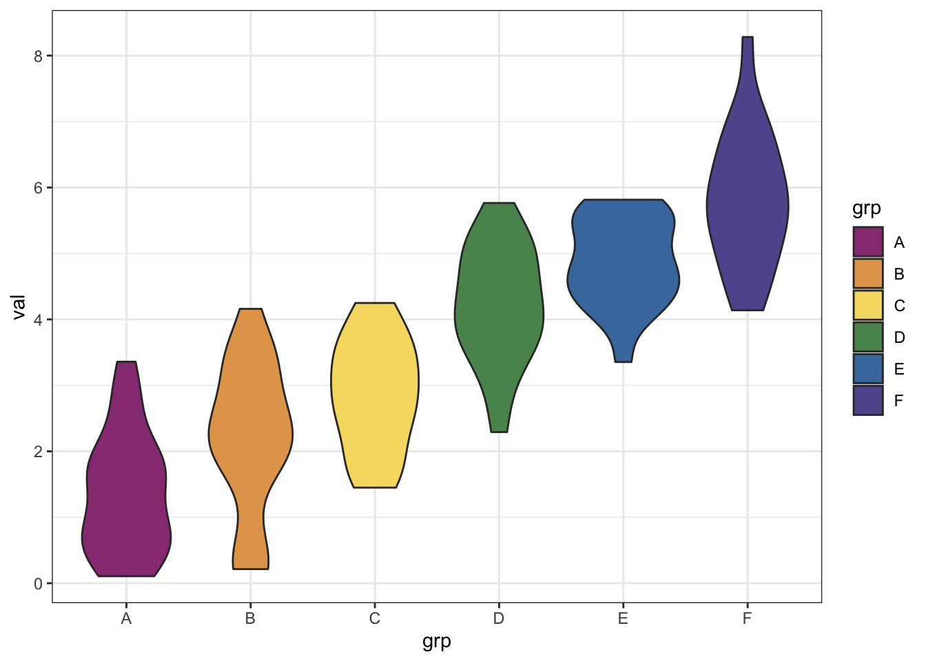
Figure 2.1: Plot with psyteachr.colours
2.5 Figures
Use \@ref(fig:chunk-name) to link to and reference the figure number in text (e.g., Figure 2.2). You can learn more about including figures and images in the Bookdown book.
The chunk label for figures can only contain alphanumeric characters (a-z, A-Z, 0-9), slashes (/), or dashes (-). Otherwise, they are not automatically numbered.
2.5.1 R Plots
Any graphs should be dynamically created in an R code block. Set echo=FALSE if you don't want to display the code that creates a plot. Default values are specified below; you don't have to include those unless you want to change them, but always set the fig.cap.
out.width='100%'fig.align='center'fig.width=8fig.height=5fig.cap='**CAPTION THIS FIGURE!!**'
```{echo=FALSE, out.width='75%', fig.width=6, fig.height=2.5, fig.cap='Dynamically created plot.'}
ggplot(iris, aes(Sepal.Length, Sepal.Width, color = Species)) +
  geom_point() +
  geom_smooth(method = lm, formula = y~x)
```
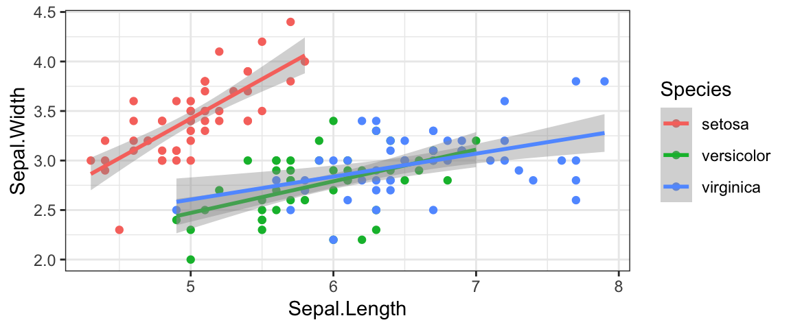
Figure 2.2: Dynamically created plot.
2.5.2 Images
Static images, like screenshots, should be stored in a directory called images and displayed using the knitr::include_graphics function in a code block.
```{r img-psyteacher-logo, echo=FALSE, fig.cap="PsyTeachR Logo"}
knitr::include_graphics("images/psyteachr_logo.png")```
Figure 2.3: PsyTeachR Logo displayed by the previous code block.
2.5.3 Screenshots
You'll probably want to include some screenshots of RStudio. For consistency, make sure your Rstudio is set to the default editor theme (Modern editor with Text-Mate theme and Consolas font). Set the font size to at least 18 for readability in screenshots.
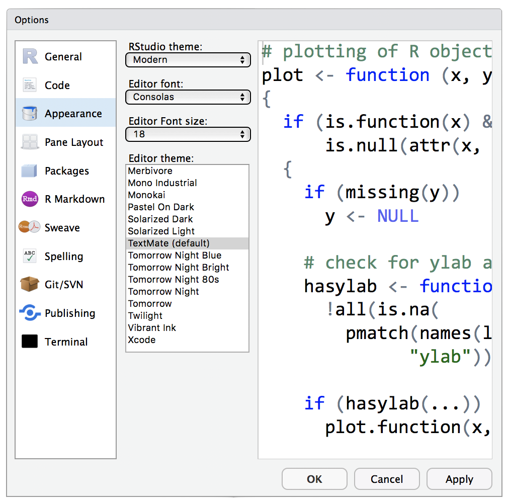
Figure 2.4: Default RStudio editor settings.
Keep panes in the default order.
- Upper left: Source
- Upper right: Environment, History, Connections, Build, Git
- Lower right: Files, Plots, Packages, Help, Viewer
- Lower left: Console
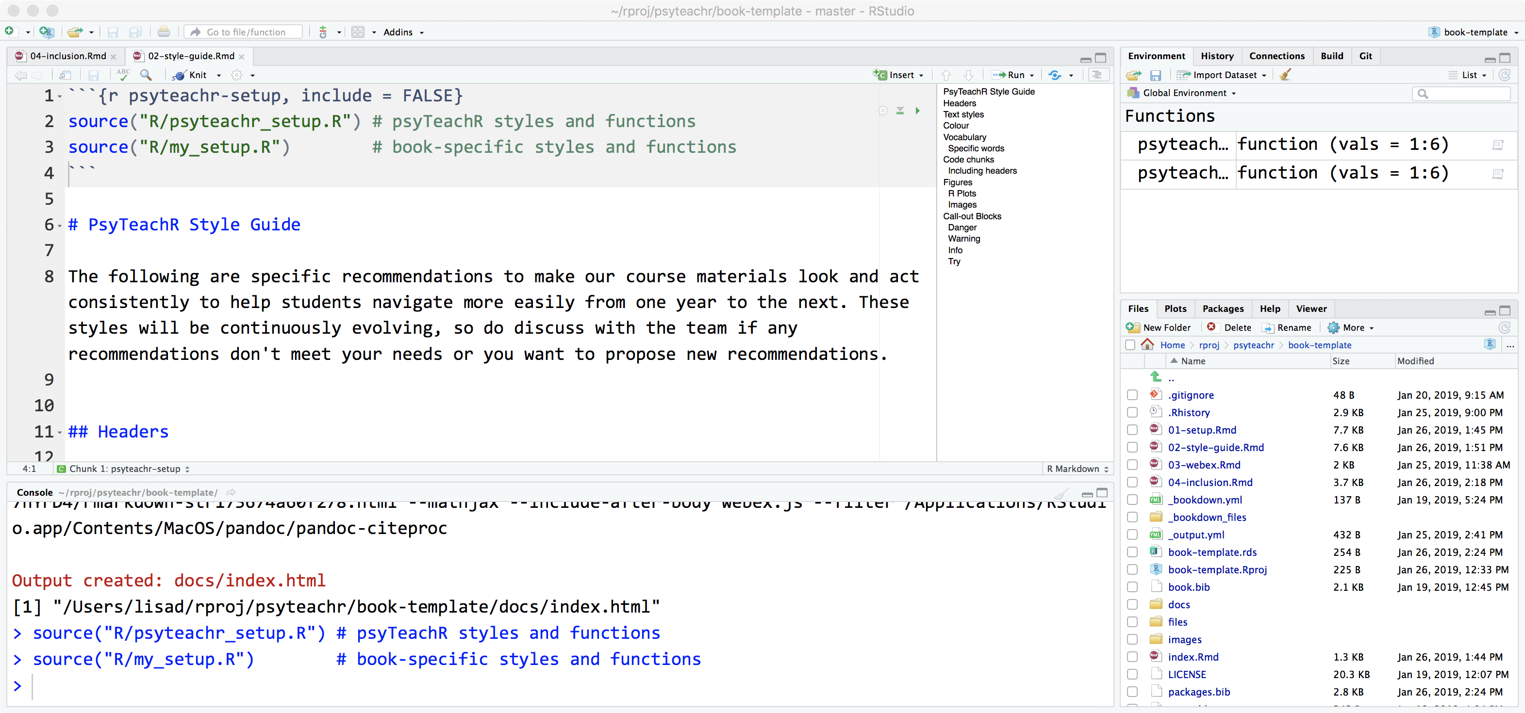
Figure 2.5: Default RStudio pane layout.
2.6 Code chunks
Always name your code chunks; this makes debugging easier and becomes the name of generated plots. You can duplicate chunk names between .Rmd files, but not within.
The chunk label for tables and figures can only contain alphanumeric characters (a-z, A-Z, 0-9), slashes (/), or dashes (-). Otherwise, they are not automatically numbered. So just get into the habit of avoiding underscores.
2.6.1 Options
Code chunks can take several options The most common ones are explained below. Learn more about code chunks.
eval: set toFALSEto skip running the codeecho: set toFALSEto skip displaying the codeinclude: set toFALSEto run but show no output (e.g., code, figures, messages, warnings)cache: set toTRUEif you have a code chunk that takes a long time to run. It should run if you make changes, but doesn't always. Delete your cache and render the book from scratch before you push major updatesresults- "hold" to hold all the output pieces and display them after the code chunk (default for psyTeachR books)
- "markup" to intersperse code and output as they happen
- "hide" to hide output
- "asis" to write raw results (like the output of
knitr::kable)
2.6.2 Including headers
If you want to show students an example of a code chunk that includes the header, add an option called verbatim to your code chunk and set it equal to what you want displayed inside the curly brackets. Make sure you set eval=FALSE to stop the code chunk from being run.
```{r verbatim-example, eval = FALSE, verbatim = 'r chunk-name, messages=FALSE'}
library(tidyverse)```
The "verbatim" option is not standard to bookdown. It is only available if you include the code from the "R/psyteachr_setup.R" file.
2.6.3 Verbatim inline backticks
Include verbatim inline r like this `r backtick("r 3+4")` to produce output like this: `r 3+4`.
2.7 Call-out Blocks
The psyTeachR course book style includes four types of call-out blocks that you can use to emphasise text.
2.7.1 Danger
```{block, type="danger"}Note dangerous things that will break code.```
Note dangerous things that will break code.
2.7.2 Warning
```{block, type="warning"}Warn readers.```
Warn readers.
2.7.3 Info
```{block, type="info"}Give further information.```
Give further information.
2.7.4 Try
```{block, type="try"}Stop and try something.```
Stop and try something.
2.7.5 Code chunks inside call-out blocks
If you want to put code blocks inside of a call-out block, you can't use the syntax above. Start the block with <div class="danger"> and end it with </div>.
<div class="danger">
Run the code below:

```r
# my code
```
</div>
2.8 References
Include references using the bibliography key, such as @R-base, which provides an in-line citation like R Core Team (2021). You can also use square brackets to create a parenthetical citation, like [@R-bookdown] (Xie 2021).
You need to add any R packages you want to cite by adding them to the code chunk in the index file and then referencing them by @R-pckgname.
# automatically create a bib database for R packages
# add any packages you want to cite here
knitr::write_bib(c(
  .packages(), 'bookdown', 'tidyverse'
), 'packages.bib')
Add other references to the book.bib file using BibTeX format. You can export references from most reference managers in BibTeX format.