E Comparing two correlations
Sometimes you will need or want to statistically compare the strength of two correlation coefficients to help determine whether they are statistically different (rather than just comparing r values). For this set of analyses you will need to install and load the cocor package as well as the tidyverse and lsr.
library(cocor)
library(tidyverse)
library(lsr)
The cocor package comes with a built-in dataset called aptitude. This dataset contains scores on four aptitude tests knowledge, logic, intelligence.a, and intelligence.b for two separate samples. This data is stored in a list object that then contains two separate data frames sample1 and sample2. We haven't worked with lists much in this book but cocor requires the data to be in list format so it's worth spending a little time on this before we get going.
First, load the built-in aptitude dataset.
data("aptitude")You can view the contents of each dataset by calling them separately:
aptitude$sample1
aptitude$sample2
However, it may that your research dataset isn't structured like this and that the data for the two groups or samples you want to compare is in the same dataset (for example, for the data for your quantitative report).
The below code transforms the data to the format you're likely to have so that we can show you how to put it back into list form by using the bind_rows() function to pull out the two datasets, bind them together, and add on a column called sample that identifies which dataset the data is from.
- Run the below code and then view
full_datto see how it is structured.
full_dat <- bind_rows(aptitude$sample1, aptitude$sample2, .id = "sample")This is how the data for your quantitative report is structured. All the data you have is in a single table and there is a column that tells you what group it is from (in this case sample but for the quant report this might be gender or whether the student is mature).
To use cocor to compare the correlations you will need to transform it into a list object. We achieve this by creating two separate objects for each sample using filter() and then we combine them back into a list. We've also added in the code to ensure that the table is a data frame because cocor is a bit fussy about what it needs.
sample1 <- full_dat %>%
  filter(sample == 1)

sample2 <- full_dat %>%
  filter(sample == 2)

dat_list <- list(sample1 = as.data.frame(sample1),
                 sample2 = as.data.frame(sample2))
This is somewhat convoluted but the key takeaway is that if you want to use cocor to compare correlations, you need to ensure your data is in a list object and that may require the above transformation.
E.0.1 Compare two correlations based on two independent groups
In this example we want to compare two correlations from two independent groups, i.e., where the participants involved in each correlation are completely different. Let's run the correlations for the full dataset, and then for sample 1 and sample 2 separately.
cor.test(full_dat$logic, full_dat$intelligence.a, method = "pearson")
cor.test(sample1$logic, sample1$intelligence.a, method = "pearson")
cor.test(sample2$logic, sample2$intelligence.a, method = "pearson")
##
## Pearson's product-moment correlation
##
## data: full_dat$logic and full_dat$intelligence.a
## t = 6.3039, df = 623, p-value = 5.497e-10
## alternative hypothesis: true correlation is not equal to 0
## 95 percent confidence interval:
## 0.1697040 0.3172053
## sample estimates:
## cor
## 0.244871
##
##
## Pearson's product-moment correlation
##
## data: sample1$logic and sample1$intelligence.a
## t = 5.7687, df = 289, p-value = 2.053e-08
## alternative hypothesis: true correlation is not equal to 0
## 95 percent confidence interval:
## 0.2142758 0.4207744
## sample estimates:
## cor
## 0.32134
##
##
## Pearson's product-moment correlation
##
## data: sample2$logic and sample2$intelligence.a
## t = 3.7665, df = 332, p-value = 0.0001958
## alternative hypothesis: true correlation is not equal to 0
## 95 percent confidence interval:
## 0.09723082 0.30316175
## sample estimates:
## cor
## 0.2024331Here we can see that the correlations between logic scores and intelligence.a scores are significant overall and in both samples separately, however, the correlation for sample 1 is larger (r = .32) than for sample 2 (r = .20) and so we can compare these using cocor.
- The left-hand side of the formula (before the
|) refers to variables in the first dataset in the list, the right-hand side of the formula (after the|) refers to variables in the second dataset in the list. - This comparison requires us to use the list object we created.
cocor(formula = ~logic + intelligence.a | logic + intelligence.a,
      data = dat_list)
##
## Results of a comparison of two correlations based on independent groups
##
## Comparison between r1.jk (logic, intelligence.a) = 0.3213 and r2.hm (logic, intelligence.a) = 0.2024
## Difference: r1.jk - r2.hm = 0.1189
## Data: sample1: j = logic, k = intelligence.a; sample2: h = logic, m = intelligence.a
## Group sizes: n1 = 291, n2 = 334
## Null hypothesis: r1.jk is equal to r2.hm
## Alternative hypothesis: r1.jk is not equal to r2.hm (two-sided)
## Alpha: 0.05
##
## fisher1925: Fisher's z (1925)
## z = 1.5869, p-value = 0.1125
## Null hypothesis retained
##
## zou2007: Zou's (2007) confidence interval
## 95% confidence interval for r1.jk - r2.hm: -0.0281 0.2637
## Null hypothesis retained (Interval includes 0)The full paper by Diedenhofen and Musch (2015) explains the output in detail, for our purposes, Fisher's z-test tells us that our correlations are not significantly different (z = 1.59, p = .113) and Zou's confidence intervals gives us the CI for the size of the difference between the two correlations (which at -0.0281 - 0.2637 is quite a range and so isn't surprising that the two are not statistically different).
E.0.1.1 Visualising two groups correlations
Rather than producing two separate scatterplots, it can be useful to display the data from bot groups on the same plot. For the dataset we have, this requires a little bit of wrangling first, if you have all the data from both groups in one object, you could skip step one.
- The
colourargument tellsggplot()to draw thegeom_jitter()andgeom_smooth()in different colours for each level ofsample. - We're using
geom_jitter()instead ofgeom_point()because many of the data points overlap - try changing it togeom_point()and see how it looks.
ggplot(full_dat, aes(x = logic, y = intelligence.a,
                         colour = sample)) +
  geom_jitter() +
  geom_smooth(method = "lm") +
  theme_minimal() +
  scale_colour_viridis_d(option = "E")
## `geom_smooth()` using formula 'y ~ x'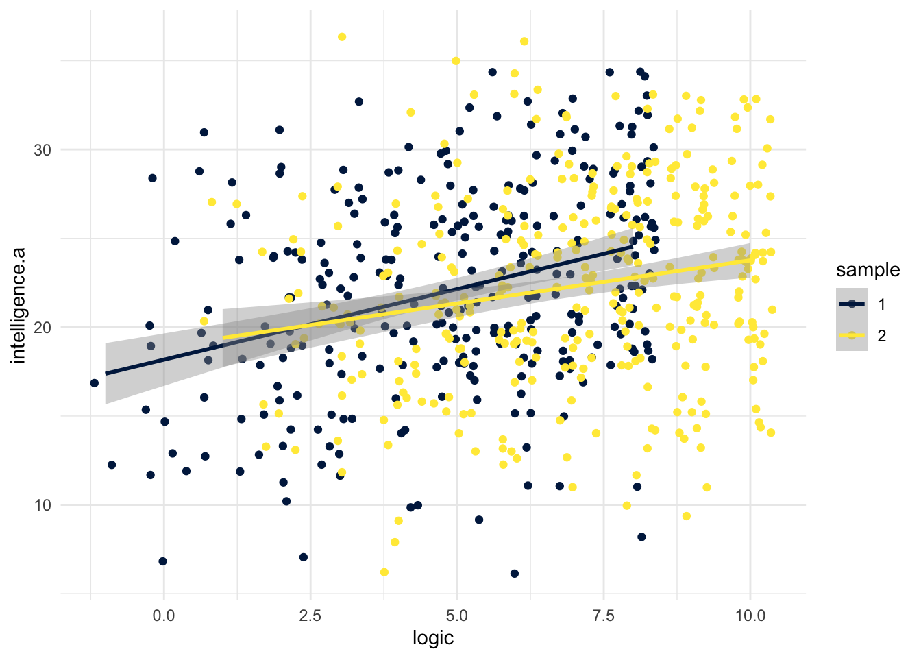
Figure 8.2: Scatterplot comparing correlation between two variables for two groups
E.0.2 Compare two overlapping correlations based on two dependent groups
In this example, we want to compare two correlations from two dependent groups (i.e., the participants are the same) and where one of the variables is also the same, i.e., it overlaps.
For example, let's run all possible correlations for sample 2:
sample2 %>%
  correlate(test = TRUE, p.adjust.method = "holm")
##
## CORRELATIONS
## ============
## - correlation type: pearson
## - correlations shown only when both variables are numeric
##
## sample knowledge logic intelligence.b
## sample . . . .
## knowledge . . 0.031 0.129.
## logic . 0.031 . 0.201***
## intelligence.b . 0.129. 0.201*** .
## intelligence.a . 0.116. 0.202*** 0.643***
## intelligence.a
## sample .
## knowledge 0.116.
## logic 0.202***
## intelligence.b 0.643***
## intelligence.a .
##
## ---
## Signif. codes: . = p < .1, * = p<.05, ** = p<.01, *** = p<.001
##
##
## p-VALUES
## ========
## - total number of tests run: 6
## - correction for multiple testing: holm
##
## sample knowledge logic intelligence.b intelligence.a
## sample . . . . .
## knowledge . . 0.567 0.055 0.068
## logic . 0.567 . 0.001 0.001
## intelligence.b . 0.055 0.001 . 0.000
## intelligence.a . 0.068 0.001 0.000 .
##
##
## SAMPLE SIZES
## ============
##
## sample knowledge logic intelligence.b intelligence.a
## sample 334 334 334 334 334
## knowledge 334 334 334 334 334
## logic 334 334 334 334 334
## intelligence.b 334 334 334 334 334
## intelligence.a 334 334 334 334 334We see that the correlations between logic, intelligence.a and intelligence.b are all significant. We can assess whether the correlation between logic and intelligence.a is strong than with intelligence.b.
- Note that the the
dataargument now specifies which dataset of the list to use. We could also have just used thesample1data that we extracted earlier.
cocor(formula = ~logic + intelligence.a | logic + intelligence.b,
      data = dat_list$sample1)
##
## Results of a comparison of two overlapping correlations based on dependent groups
##
## Comparison between r.jk (logic, intelligence.a) = 0.3213 and r.jh (logic, intelligence.b) = 0.2679
## Difference: r.jk - r.jh = 0.0534
## Related correlation: r.kh = 0.4731
## Data: dat_list$sample1: j = logic, k = intelligence.a, h = intelligence.b
## Group size: n = 291
## Null hypothesis: r.jk is equal to r.jh
## Alternative hypothesis: r.jk is not equal to r.jh (two-sided)
## Alpha: 0.05
##
## pearson1898: Pearson and Filon's z (1898)
## z = 0.9419, p-value = 0.3462
## Null hypothesis retained
##
## hotelling1940: Hotelling's t (1940)
## t = 0.9422, df = 288, p-value = 0.3469
## Null hypothesis retained
##
## williams1959: Williams' t (1959)
## t = 0.9379, df = 288, p-value = 0.3491
## Null hypothesis retained
##
## olkin1967: Olkin's z (1967)
## z = 0.9419, p-value = 0.3462
## Null hypothesis retained
##
## dunn1969: Dunn and Clark's z (1969)
## z = 0.9370, p-value = 0.3487
## Null hypothesis retained
##
## hendrickson1970: Hendrickson, Stanley, and Hills' (1970) modification of Williams' t (1959)
## t = 0.9422, df = 288, p-value = 0.3469
## Null hypothesis retained
##
## steiger1980: Steiger's (1980) modification of Dunn and Clark's z (1969) using average correlations
## z = 0.9367, p-value = 0.3489
## Null hypothesis retained
##
## meng1992: Meng, Rosenthal, and Rubin's z (1992)
## z = 0.9365, p-value = 0.3490
## Null hypothesis retained
## 95% confidence interval for r.jk - r.jh: -0.0640 0.1811
## Null hypothesis retained (Interval includes 0)
##
## hittner2003: Hittner, May, and Silver's (2003) modification of Dunn and Clark's z (1969) using a backtransformed average Fisher's (1921) Z procedure
## z = 0.9367, p-value = 0.3489
## Null hypothesis retained
##
## zou2007: Zou's (2007) confidence interval
## 95% confidence interval for r.jk - r.jh: -0.0583 0.1649
## Null hypothesis retained (Interval includes 0)This produces a large number of tests, the mathematics of which are described in the cocor documentation.. The cocor documentation suggests basing the decision on convergence - in this case all tests indicated the null hypothesis should be retained, i.e., the correlations are not significantly different. For the purposes of writing up such a comparison, [Silver, Hittner & May (2004)]((https://www.tandfonline.com/doi/abs/10.3200/JEXE.71.1.53-70) suggest that Dunn & Clark's performs best so you can report that (z = .94, p = .349) as well as Zou's confidence intervals.
E.0.3 Compare two non-overlapping correlations from two dependent groups
The final comparison we could make is to compare two non-overlapping (none of the variables are the same) correlations from two dependent groups (the same sample).
cocor(formula = ~logic + intelligence.b | knowledge + intelligence.a,
      data = dat_list$sample1)
##
## Results of a comparison of two nonoverlapping correlations based on dependent groups
##
## Comparison between r.jk (logic, intelligence.b) = 0.2679 and r.hm (knowledge, intelligence.a) = 0.1038
## Difference: r.jk - r.hm = 0.164
## Related correlations: r.jh = 0.0257, r.jm = 0.3213, r.kh = 0.1713, r.km = 0.4731
## Data: dat_list$sample1: j = logic, k = intelligence.b, h = knowledge, m = intelligence.a
## Group size: n = 291
## Null hypothesis: r.jk is equal to r.hm
## Alternative hypothesis: r.jk is not equal to r.hm (two-sided)
## Alpha: 0.05
##
## pearson1898: Pearson and Filon's z (1898)
## z = 2.0998, p-value = 0.0357
## Null hypothesis rejected
##
## dunn1969: Dunn and Clark's z (1969)
## z = 2.0811, p-value = 0.0374
## Null hypothesis rejected
##
## steiger1980: Steiger's (1980) modification of Dunn and Clark's z (1969) using average correlations
## z = 2.0755, p-value = 0.0379
## Null hypothesis rejected
##
## raghunathan1996: Raghunathan, Rosenthal, and Rubin's (1996) modification of Pearson and Filon's z (1898)
## z = 2.0811, p-value = 0.0374
## Null hypothesis rejected
##
## silver2004: Silver, Hittner, and May's (2004) modification of Dunn and Clark's z (1969) using a backtransformed average Fisher's (1921) Z procedure
## z = 2.0753, p-value = 0.0380
## Null hypothesis rejected
##
## zou2007: Zou's (2007) confidence interval
## 95% confidence interval for r.jk - r.hm: 0.0095 0.3162
## Null hypothesis rejected (Interval does not include 0)Again the output produces a number of tests, although in this case they all converge on the conclusion that the null hypothesis should be rejected, i.e., the correlations are significantly different. Again following Silver et al., if you need to pick one to report, I'd suggest Dunn and Clark's z with Zou's confidence intervals.