Chapter 15 Factorial ANOVA

For the second week of ANOVA we're going to look at an example of a factorial ANOVA. You'll learn more about interpreting these in the second lecture, but for now, we'll just focus on the code.

We're going to reproduce the analysis from Experiment 3 of Zhang, T., Kim, T., Brooks, A. W., Gino, F., & Norton, M. I. (2014). A "present" for the future: The unexpected value of rediscovery. Psychological Science, 25, 1851-1860.. You may remember this study from the Chapter Visualisation chapter.

This experiment has a 2 x 2 mixed design:

The first IV is time (time1, time2) and is within-subjects
The second IV is type of event (ordinary vs. extraordinary) and is a between-subjects factor
The DV we will use is interest

15.0.1 Activity 1: Set-up

Open R Studio and set the working directory to your chpter folder. Ensure the environment is clear.
Open a new R Markdown document and save it in your working directory. Call the file "Factorial ANOVA".
Download Zhang et al. 2014 Study 3.csv and extract the files in to your Week 11 folder.
If you're on the server, avoid a number of issues by restarting the session - click Session - Restart R
If you are working on your own computer, install the package rcompanion. Remember do not install packages on university computers, they are already installed.
Type and run the code that loads pwr, rcompanion, lsr, car, broom, afex, emmeans and tidyverse using the library() function.

Run the below code to load the data and wrangle it into the format we need. You don't need to write this code yourself but do make sure you can understand what each line is doing - a good way to do this when the code uses pipes (%>%) is to highlight and run each line progressively so you can see how it builds up. Line-by-line the code:

Reads in the data file
Select the three columns we need
Adds on a column of subject IDs
Tidies the data
Recodes the values of Condition from numeric to text labels
Recodes the values of time to be easier to read/write

factorial <- read_csv("Zhang et al. 2014 Study 3.csv")%>%
  select(Condition, T1_Predicted_Interest_Composite, T2_Actual_Interest_Composite)%>%
  mutate(subject = row_number())%>%
  pivot_longer(names_to = "time",values_to = "interest", cols =       c("T1_Predicted_Interest_Composite","T2_Actual_Interest_Composite"))%>%
  mutate(Condition = dplyr::recode(Condition, "1" = "Ordinary", "2" = "Extraordinary"))%>%
  mutate(time = dplyr::recode(time, "T1_Predicted_Interest_Composite" = "time1_interest",
                       "T2_Actual_Interest_Composite" = "time2_interest")) %>%
  mutate(Condition = as.factor(Condition))

15.0.2 Activity 2: Descriptive statistics

Calculate descriptive statistics (mean and SD) for interest for each Condition for each time (hint: you will need to group_by() two variables) and store it in an object named sum_dat_factorial. These are known as the cells means.

15.0.3 Activity 3: Violin-boxplots

We're going to produce two kinds of plots to visualise our data. First, we'll produce violin-boxplots so that we can see the distribution of our data.

Write the code that produces the below violin-boxplots for the scores in each group.
- Hint 1: you will need to add in the second IV in the first call to ggplot as a fill argument (aes(x,y,fill)).
- Hint 2: you will need to add position = position_dodge(.9) to geom_boxplot to get the plots to align.

You don't need to replicate the exact colour scheme used below, see if you can play around with the settings to whatever colour scheme you think works best.

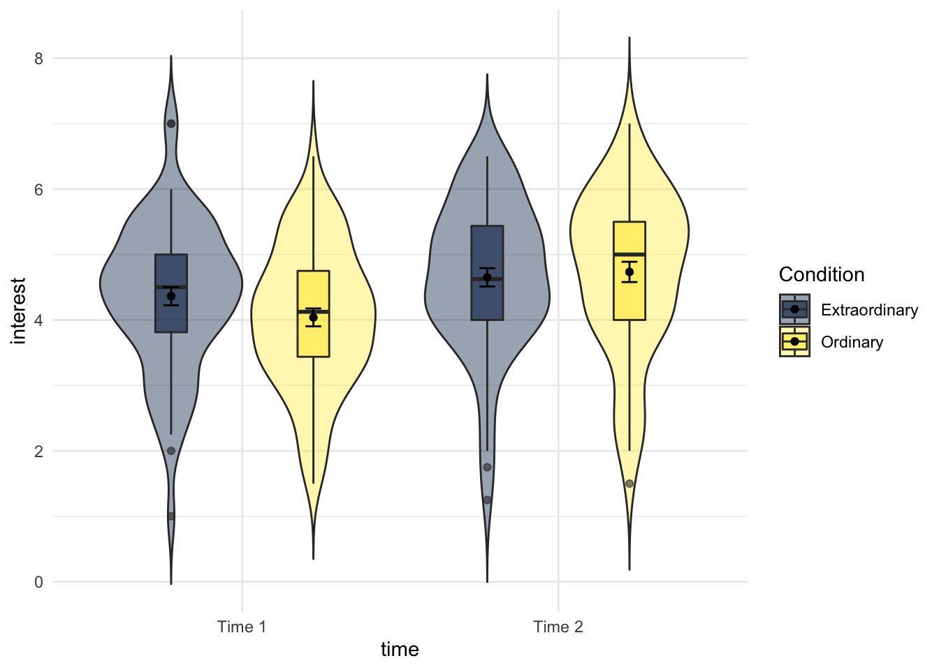
Figure 15.1: Violin-boxplot by condition and time

15.0.4 Activity 4: Interaction plots

Now we're going to produce an interaction plot that makes it easier to see how the IVs are interacting, which requires some ggplot2 functions we haven't come across yet. Rather than using the raw data in dat_factorial, we use the means that we produced in sum_dat_factorial. This type of plot requires two geoms, one to draw the points, and one to draw the lines that connect them.

This plot reproduces the plot used in the paper.

Run the code and then play around with how it looks by changing the arguments for e.g., colour, line-type, and the theme.

ggplot(sum_dat_factorial, aes(x = time, y = mean, group = Condition, shape = Condition)) +
  geom_point(size = 3) +
  geom_line(aes(linetype = Condition))+
  scale_x_discrete(labels = c("Time 1", "Time 2"))+
  theme_classic()

Figure 15.2: Interaction plot

15.0.5 Activity 5: ANOVA

Complete the below code to run the factorial ANOVA. Remember that you will need to specify both IVs and that one of them is between-subjects and one of them is within-subjects. Look up the help documentation for aov_ez to find out how to do this.
Save the ANOVA model to an object called mod_factorial
Pull out the anova table, you can either do this with mod_factorial$anova_table or anova(mod_factorial) both have the same result. Save this to an object named factorial_output and make sure you have used tidy().

mod_factorial <- aov_ez(id = "NULL",
               data = NULL, 
               between = "NULL", 
               within = "NULL",
               dv = "NULL", 
               type = 3,
               es = "NULL") 

factorial_output <- NULL

Look at the results. Remember the pre-class information about how to read p-values in scientific notation.

Is the main effect of condition significant?
Is the main effect of time significant?
Is the two-way interaction significant?

15.0.6 Activity 6: Assumption checking

The assumptions for a factorial ANOVA are the same as the one-way ANOVA.

The DV is interval or ratio data
The observations should be independent
The residuals should be normally distributed
There should be homogeneity of variance between the groups

As before, we know assumption 2 is met from the design of the study. Assumption 1 throws up an interesting issue which is the problem of ordinal data. Ordinal data is the kind of data that comes from Likert scales and is very, very common in psychology. The problem is that ordinal data isn't interval or ratio data, there's a fixed number of values it can take (the values of the Likert scale) and you can't claim that the distance between the values is equal (is the difference between strongly agree and agree the same as the difference between agree and neutral?).

Technically, we shouldn't use an ANOVA to analyse ordinal data - but almost everyone does. Most people would argue that if there are multiple Likert scale items that are averaged (which is the case in our study) and this averaged data is normally distributed, then it is not a problem. There is a minority (who are actually correct) that argue you should use non-parametric methods or more complicated tests such as ordinal regression for this type of data. Whichever route you choose, you should understand the data you have and you should be able to justify your decision.

To test assumption 3, extract the residuals from the model (mod_factorial$lm$residuals), create a qq-plot and conduct a Shapiro-Wilk test.
Are the residuals normally distributed?

For the final assumption, we can again use test_levene() to test homogeneity of variance.

Conduct Levene's test. Is assumption 4 met?

15.0.7 Activity 7: Post-hoc tests

Because the interaction is significant, we should follow this up with post-hoc tests using emmeans() to determine which comparisons are significant. If the overall interaction is not significant, you should not conduct additional tests.

emmeans() requires you to specify the aov object, and then the factors you want to contrast. For an interaction, we use the notation pairwise ~ IV1 | IV2 and you specify which multiple comparison correction you want to apply. Finally, you can use tidy() to tidy up the output of the contrasts and save it into a tibble.

Run the below code and view the results.

# run the tests
posthoc_factorial <- emmeans(mod_factorial$aov, 
                             pairwise ~ time| Condition, 
                             adjust = "bonferroni")

# tidy up the output of the tests
contrasts_factorial <- posthoc_factorial$contrasts %>%
  tidy()

Note that because there are two factors, we could also reverse the order of the IVs. Above, we get the results contrasting time 1 and time 2 for each condition. Instead, we could look at the difference between ordinary and extraordinary events at each time point.

Run the below code and look at the output of contrast_factorial and contrasts_factorial2 carefully making sure you understand how to interpret the results. You will find it useful to refer to the interaction plot we made earlier.

posthoc_factorial2 <- emmeans(mod_factorial$aov, 
                             pairwise ~ Condition| time, 
                             adjust = "bonferroni") 

contrasts_factorial2 <- posthoc_factorial2$contrasts %>%
  tidy()

Because our main effects (condition and time) only have two levels, we don't need to do any post-hoc tests to determine which conditions differ from each other, however, if one of our factors had three levels then we could use emmeans() to calculate the contrast for the main effects, like we did for the one-way ANOVA.

Finally, to calculate effect size for the pairwise comparisons we again need to do this individually using 'cohensD()fromlsr`.

Run the below code to add on effect sizes to contrasts_factorial and contrasts_factorial2.

d_extra_t1_t2 <- cohensD(interest ~ time, 
                         data = (filter(factorial, Condition == "Extraordinary") %>% droplevels())) 

d_ord_t1_t2 <- cohensD(interest ~ time, 
                         data = (filter(factorial, Condition == "Ordinary") %>% droplevels())) 


Condition_ds <- c(d_extra_t1_t2, d_ord_t1_t2)

contrasts_factorial <- contrasts_factorial %>%
  mutate(eff_size = Condition_ds)

d_time1_extra_ord <- cohensD(interest ~ Condition, 
                         data = (filter(factorial, time == "time1_interest") %>% droplevels())) 

d_time2_extra_ord <- cohensD(interest ~ Condition, 
                         data = (filter(factorial, time == "time2_interest") %>% droplevels()))


time_ds <- c(d_time1_extra_ord, d_time2_extra_ord)

contrasts_factorial2 <- contrasts_factorial %>%
  mutate(eff_size = time_ds)

15.0.8 Activity 8: Write-up

p-values of < .001 have been entered manually. There is a way to get R to produce this formatting but it's overly complicated for our purposes. If you want to push yourself, look up the papaja package.
The values of partial eta-squared do not match between our analysis and those reported in the paper. I haven't figured out why this is yet - if you know, please get in touch!
We have replaced the simple effects in the main paper with our pairwise comparisons.

First we need to calculate descriptives for the main effect of time as we didn't do this earlier.

time_descrip <- factorial %>% 
  group_by(time) %>%
  summarise(mean_interest = mean(interest, na.rm = TRUE),
            sd_interest = sd(interest, na.rm = TRUE),
            min = mean(interest) - qnorm(0.975)*sd(interest)/sqrt(n()),
            max = mean(interest) + qnorm(0.975)*sd(interest)/sqrt(n()))

Copy and paste the below into white-space.

We conducted the same repeated measures ANOVA with interest as the dependent measure and again found a main effect of time, F(`r factorial_output$num.Df[2]`, `r factorial_output$den.Df[2]`) = `r factorial_output$statistic[2] %>% round(2)`, p < .001, ηp2 = `r factorial_output$ges[2] %>% round(3)`; anticipated interest at Time 1 (M = `r time_descrip$mean_interest[1] %>% round(2)`), SD = `r time_descrip$sd_interest[1]%>% round(2)`)) was lower than actual interest at Time 2 (M = `r time_descrip$mean_interest[2]%>% round(2)`, SD = `r time_descrip$sd_interest[2]%>% round(2)`).We also observed an interaction between time and type of experience, F(`r factorial_output$num.Df[3]`, `r factorial_output$den.Df[3]`) = `r factorial_output$statistic[3] %>% round(3)`, p = `r factorial_output$p.value[3] %>% round(2)`, ηp2 = `r factorial_output$ges[3] %>% round(3)`. Pairwise comparisons revealed that for ordinary events, predicted interest at Time 1 (M = `r sum_dat_factorial$mean[3]%>% round(2)`, SD = `r sum_dat_factorial$sd[3]%>% round(2)`) was lower than experienced interest at Time 2 (M = `r sum_dat_factorial$mean[4]%>% round(2)`, SD = `r sum_dat_factorial$sd[4]%>% round(2)`), t(`r contrasts_factorial$df[2]%>% round(2)`) = `r contrasts_factorial$statistic[2]%>% round(2)`, p < .001, d = `r contrasts_factorial$eff_size[2]%>% round(2)`. Although predicted interest for extraordinary events at Time 1 (M = `r sum_dat_factorial$mean[1]%>% round(2)`, SD = `r sum_dat_factorial$sd[1]%>% round(2)`) was lower than experienced interest at Time 2 (M = `r sum_dat_factorial$mean[2]%>% round(2)`, SD = `r sum_dat_factorial$sd[2]%>% round(2)`), t(`r contrasts_factorial$df[1]%>% round(2)`) = `r contrasts_factorial$statistic[1]%>% round(2)`, p < .001, d = `r contrasts_factorial$eff_size[1]%>% round(2)` , the magnitude of underestimation was smaller than for ordinary events.

We conducted the same repeated measures ANOVA with interest as the dependent measure and again found a main effect of time, F(1, 128) = 25.88, p < .001, ηp2 = 0.044; anticipated interest at Time 1 (M = 4.2), SD = 1.12)) was lower than actual interest at Time 2 (M = 4.69, SD = 1.19).We also observed an interaction between time and type of experience, F(1, 128) = 4.445, p = 0.04, ηp2 = 0.008. Pairwise comparisons revealed that for ordinary events, predicted interest at Time 1 (M = 4.04, SD = 1.09) was lower than experienced interest at Time 2 (M = 4.73, SD = 1.24), t(128) = -5.05, p < .001, d = 0.59. Although predicted interest for extraordinary events at Time 1 (M = 4.36, SD = 1.13) was lower than experienced interest at Time 2 (M = 4.65, SD = 1.14), t(128) = -2.12, p < .001, d = 0.25 , the magnitude of underestimation was smaller than for ordinary events.

15.0.9 Activity 9: Transforming data

In this chapter we decided that the violation of the assumption of normality was ok so that we could replicate the results in the paper. But what if we weren't happy with this or if the violation had been more extreme? One option to deal with normality is to transform your data. If you want more information on this you should consult the Appendix chapter on data transformation.

There are various options for how you can transform data but we're going to use Tukeys Ladder of Powers transformation. This finds the power transformation that makes the data fit the normal distribution as closely as possible with this type of transformation.

Run the below code. This will use mutate() to add a new variable to the data-set, interest_tukey which is going to be our transformed DV. The function transformTukey() is from the rcompanion package. Setting plotit = TRUE will automatically create qqPlots and histograms so that we can immediately visualise the new variable.

factorial <- factorial %>%
  mutate(interest_tukey = transformTukey(interest, plotit=TRUE))

Now that you've transformed the DV we can re-run the ANOVA with this new variable.

tukey_factorial <- aov_ez(id = "subject",
               data = factorial, 
               between = "Condition", 
               within = "time",
               dv = "interest_tukey", 
               type = 3)

tukey_factorial

Notice that doing this hasn't changed the pattern of the ANOVA results, the p-values for the main effects and interactions are very slightly different but the overall conclusions remain the same. This is likely because the violations of normality was quite mild and there is a large sample size, however, with the transformation we can be more confident in our results and it may not always be the case that the transformed ANOVA is the same if the violations were more extreme.

15.0.9.1 Finished!

And we're done! There's only one more week of R left. I know that for some of you, you will be breathing a sigh of relief but we really want you to reflect on just how far you've come and the skills that you've learned. Even if you don't continue with quantitative research, your understanding of how data is manipulated and how the final results of journal articles actually happen will have substantially increased and that level of critical awareness is an all-round good skill to have.