H Non-parametric tests
First, before Dale Barr shouts at me, it needs to be noted that non-parametric tests are problematic. Because they are based on rank data:
- They ignore the magnitude of any differences therefore
- They are less powerful
- You cannot calculate interactions
Additionally, with large sample sizes the parametric options (t-tests, one-way ANOVA, Pearson's correlations) are usually robust and perform better and with the wealth of packages and tests available in R, we now all have easy access to better alternatives such as ordinal regression or permutation test, or options for data transformation that were more difficult when these tests were first popularised.
However, the textbooks still teach them and there may be situations in which you are called to perform non-parametric tests, so here we are.
H.0.0.1 Two independent groups
The non-parametric equivalent of a independent-samples t-test is known as the Mann-Whitney-U test also referred to as the Wilcoxon Rank Sum test. It uses ranked data to test the null hypothesis that the median ranks of two groups are different.
For this example we're going to use the wine dataset from the ordinal package that has ratings for different wines.
library(tidyverse)
library(ordinal)
##
## Attaching package: 'ordinal'## The following object is masked from 'package:dplyr':
##
## slicedata(wine)
force(wine)## response rating temp contact bottle judge
## 1 36 2 cold no 1 1
## 2 48 3 cold no 2 1
## 3 47 3 cold yes 3 1
## 4 67 4 cold yes 4 1
## 5 77 4 warm no 5 1
## 6 60 4 warm no 6 1
## 7 83 5 warm yes 7 1
## 8 90 5 warm yes 8 1
## 9 17 1 cold no 1 2
## 10 22 2 cold no 2 2
## 11 14 1 cold yes 3 2
## 12 50 3 cold yes 4 2
## 13 30 2 warm no 5 2
## 14 51 3 warm no 6 2
## 15 90 5 warm yes 7 2
## 16 70 4 warm yes 8 2
## 17 36 2 cold no 1 3
## 18 50 3 cold no 2 3
## 19 42 3 cold yes 3 3
## 20 23 2 cold yes 4 3
## 21 80 5 warm no 5 3
## 22 81 5 warm no 6 3
## 23 73 4 warm yes 7 3
## 24 62 4 warm yes 8 3
## 25 46 3 cold no 1 4
## 26 27 2 cold no 2 4
## 27 48 3 cold yes 3 4
## 28 32 2 cold yes 4 4
## 29 57 3 warm no 5 4
## 30 37 2 warm no 6 4
## 31 84 5 warm yes 7 4
## 32 58 3 warm yes 8 4
## 33 26 2 cold no 1 5
## 34 45 3 cold no 2 5
## 35 61 4 cold yes 3 5
## 36 41 3 cold yes 4 5
## 37 48 3 warm no 5 5
## 38 41 3 warm no 6 5
## 39 58 3 warm yes 7 5
## 40 55 3 warm yes 8 5
## 41 46 3 cold no 1 6
## 42 30 2 cold no 2 6
## 43 54 3 cold yes 3 6
## 44 37 2 cold yes 4 6
## 45 32 2 warm no 5 6
## 46 60 4 warm no 6 6
## 47 88 5 warm yes 7 6
## 48 73 4 warm yes 8 6
## 49 13 1 cold no 1 7
## 50 19 1 cold no 2 7
## 51 31 2 cold yes 3 7
## 52 29 2 cold yes 4 7
## 53 22 2 warm no 5 7
## 54 43 3 warm no 6 7
## 55 32 2 warm yes 7 7
## 56 49 3 warm yes 8 7
## 57 25 2 cold no 1 8
## 58 32 2 cold no 2 8
## 59 39 2 cold yes 3 8
## 60 40 3 cold yes 4 8
## 61 51 3 warm no 5 8
## 62 45 3 warm no 6 8
## 63 42 3 warm yes 7 8
## 64 67 4 warm yes 8 8
## 65 12 1 cold no 1 9
## 66 29 2 cold no 2 9
## 67 47 3 cold yes 3 9
## 68 28 2 cold yes 4 9
## 69 47 3 warm no 5 9
## 70 38 2 warm no 6 9
## 71 72 4 warm yes 7 9
## 72 65 4 warm yes 8 9Each wine is given a bitterness rating on a 0-100 scale (response variable) and one of the grouping variables is whether the wine was served cold or warm (temp).
First, we can calculate descriptive statistics. For ordinal data the median and range are most suitable.
wine %>%
  group_by(temp) %>%
  summarise(median_response = median(response),
            min_response = min(response),
            max_response = max(response))
## # A tibble: 2 x 4
## temp median_response min_response max_response
## <fct> <dbl> <dbl> <dbl>
## 1 cold 36 12 67
## 2 warm 58 22 90And to visualise, grouped histograms:
ggplot(wine, aes(x = response, fill = temp)) +
  geom_histogram(colour = "black",alpha = .8) +
  scale_fill_viridis_d(option = "E") +
  theme_minimal()
## `stat_bin()` using `bins = 30`. Pick better value with `binwidth`.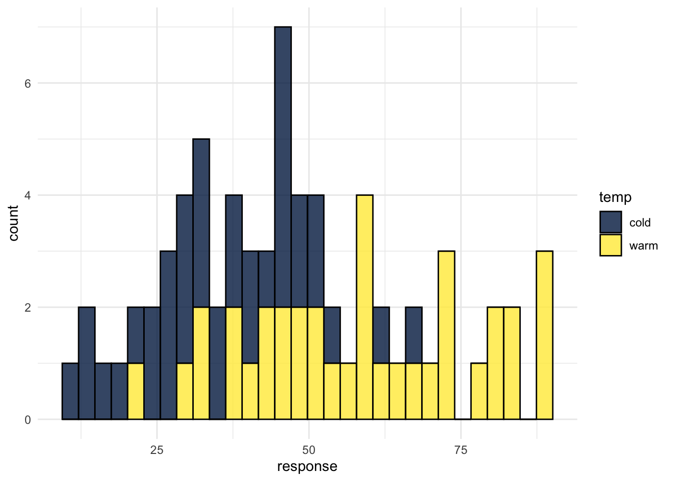
Figure H.1: CAPTION THIS FIGURE!!
The Mann-Whitney code takes the following form:
wilcox.test(dv ~ iv, data, paired = FALSE, correct = TRUE)Therefore to test whether bitterness ratings are significantly different between temperate groups.
np_test1 <- wilcox.test(response ~ temp,
            data = wine,
            paired = FALSE,
            correct = TRUE)
## Warning in wilcox.test.default(x = c(36, 48, 47, 67, 17, 22, 14, 50, 36, :
## cannot compute exact p-value with tiesnp_test1##
## Wilcoxon rank sum test with continuity correction
##
## data: response by temp
## W = 214.5, p-value = 1.072e-06
## alternative hypothesis: true location shift is not equal to 0The result of the test tells us that there is a significance difference between the groups, however, there's also a warning message about the calculation of the p-value.
When we calculate a p-value, we do it under the assumption that the data are normally distributed so that we know what the probability of getting a particular score would be. However, non-parametric data isn’t normally distributed, that's the point.
There are two solutions. First, there’s the exact method or the Monte Carlo method. This takes the data and randomizes the group labels, so it mixes up which group each score is in. It does this thousands of times to calculate the probability of the observed result - if you still get the same difference in scores between the groups when the labels have been randomly shuffled, you'd want to accept the null hypothesis.
The great thing about this method is because it randomizes the data thousands of times, you get the exact probability of your observed data. The problem is that it doesn’t work when you’ve got ties in your data.
The other way is to use the normal approximation and this is where rather than using the distribution of the data, it assumes that the distribution of the test statistic, so in this case W, is normally distributed, and calculates the probability the observed test statistic. Because the normal distribution is smooth, whereas ranked data increases in increments of .5 and 1, this can reduce the p-values so by default a correction is applied to counteract this which is what the continuity correction refers to.
H.0.0.1.1 Effect size
The effect size for a Mann-wWitney is actually pearson’s R, the same r we use in correlation and is calculated by extracting the z score from the p-value. First, we create a new function to do this for us (from Field et al., 2013) that specifies we want to calculate r for the Mann-Whitney test we stored in np_test:
rFromWilcox <-  function(np_test1, N){
  Z <- qnorm(np_test1$p.value/2)
  r <- Z/sqrt(N)
  cat(np_test1$data.name, "Effect Size, r = ", r)
}
Next, we use this new function to calculate the effect size by specifying the model object and the sample size.:
rFromWilcox(np_test1, 72)## response by temp Effect Size, r = -0.5748666H.0.0.2 APA write-up
A Mann-Whitney U test found that cold wines recieved significantly higher bitterness ratings than warm wines (W = 214.5, p <.001, r = -.58).
H.0.0.3 Spearman's correlations
The cocor package comes with a dataset called aptitude. This dataset contains scores on four aptitude tests knowledge, logic, intelligence.a, and intelligence.b for two separate samples and we'll also load lsr for correlations
library(cocor)
library(tidyverse)
library(lsr)
First, let's load the full dataset and then pull out just the data for one sample.
data(aptitude)
sample1 <- aptitude$sample1
We can use ggplot() to look at the distributions of the data. Looking at all four variables, we might conclude that the distributions for intelligence.b and logic do not meet the assumption of normality as so we want to do a non-parametric Spearman's correlation (although if N > 100, Spearman and Pearson correlations are basically identical but let's ignore that for now).
sample1 %>%
  mutate(subject = row_number()) %>%
  pivot_longer(cols = knowledge:intelligence.a, names_to = "test", values_to = "score") %>%
  ggplot(aes(x = score)) +
  geom_histogram() +
  facet_wrap(~test, scales = "free_x")
## `stat_bin()` using `bins = 30`. Pick better value with `binwidth`.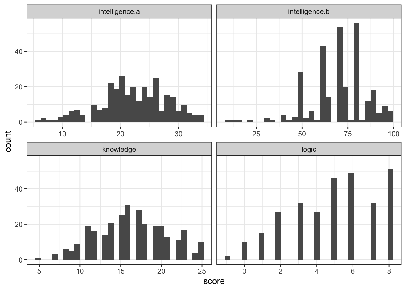
Figure H.2: CAPTION THIS FIGURE!!
To run a single Spearman's correlation we can use cor.test(). The code is the same as we have used previously with one edit, we change method to spearman.
cor.test(sample1$knowledge, sample1$logic, method = "spearman")## Warning in cor.test.default(sample1$knowledge, sample1$logic, method =
## "spearman"): Cannot compute exact p-value with ties##
## Spearman's rank correlation rho
##
## data: sample1$knowledge and sample1$logic
## S = 3999856, p-value = 0.6577
## alternative hypothesis: true rho is not equal to 0
## sample estimates:
## rho
## 0.02608352For reasons I am unclear about, the Spearman test doesn't produce degrees of freedom, the easiest way to do this is probably just to run the test again using method = "pearson" and take the DF from there.
cor.test(sample1$knowledge, sample1$logic, method = "pearson")##
## Pearson's product-moment correlation
##
## data: sample1$knowledge and sample1$logic
## t = 0.43664, df = 289, p-value = 0.6627
## alternative hypothesis: true correlation is not equal to 0
## 95 percent confidence interval:
## -0.0895695 0.1402433
## sample estimates:
## cor
## 0.02567615If you want to run multiple correlations using correlate() from lsr, again, you just need to amend the method.
sample1 %>%
  correlate(test = TRUE, corr.method = "spearman")
##
## CORRELATIONS
## ============
## - correlation type: spearman
## - correlations shown only when both variables are numeric
##
## knowledge logic intelligence.b intelligence.a
## knowledge . 0.026 0.169* 0.101
## logic 0.026 . 0.279*** 0.305***
## intelligence.b 0.169* 0.279*** . 0.486***
## intelligence.a 0.101 0.305*** 0.486*** .
##
## ---
## Signif. codes: . = p < .1, * = p<.05, ** = p<.01, *** = p<.001
##
##
## p-VALUES
## ========
## - total number of tests run: 6
## - correction for multiple testing: holm
## - WARNING: cannot compute exact p-values with ties
##
## knowledge logic intelligence.b intelligence.a
## knowledge . 0.658 0.011 0.171
## logic 0.658 . 0.000 0.000
## intelligence.b 0.011 0.000 . 0.000
## intelligence.a 0.171 0.000 0.000 .
##
##
## SAMPLE SIZES
## ============
##
## knowledge logic intelligence.b intelligence.a
## knowledge 291 291 291 291
## logic 291 291 291 291
## intelligence.b 291 291 291 291
## intelligence.a 291 291 291 291H.0.0.4 APA write-up
A Spearman’s correlation found a weak,non-significant, positive correlation (rs (289) = .03, p = .658) between knowledge and logic test scores.