Chapter 8 Probability
8.1 Activity 1: Prep
The first half of this chapter doesn't contain any coding, instead, we're going to recap some core statistical concepts. If you need any additional resources beyond what has been discussed in the lectures, you may find the below useful.
- Read Statistical thinking (Noba Project)
- Watch Normal Distribution - Explained Simply (10 mins)
- Watch Probability explained (8 mins)
- Watch Binomial distribution (12 minutes)
8.2 What is probability?
Probability (p) is the extent to which an event is likely to occur and is represented by a number between 0 and 1. For example, the probability of flipping a coin and it landing on 'heads' would be estimated at p = .5, i.e., there is a 50% chance of getting a head when you flip a coin. Calculating the probability of any discrete event occurring can be formulated as:
\[p = \frac{number \ of \ ways \ the \ event \ could \ arise}{number \ of \ possible \ outcomes}\] For example, what is the probability of randomly drawing your name out of a hat of 12 names where one name is definitely yours?
1/12## [1] 0.08333333The probability is .08, or to put it another way, there is an 8.3% chance that you would pull your name out of the hat.
8.3 Types of data
How you tackle probability depends on the type of data/variables you are working with (i.e. discrete or continuous). This is also referred to as Level of Measurements.
Discrete data can only take integer values (whole numbers). For example, the number of participants in an experiment would be discrete - we can't have half a participant! Discrete variables can also be further broken down into nominal and ordinal variables.
Ordinal data is a set of ordered categories; you know which is the top/best and which is the worst/lowest, but not the difference between categories. For example, you could ask participants to rate the attractiveness of different faces based on a 5-item Likert scale (very unattractive, unattractive, neutral, attractive, very attractive). You know that very attractive is better than attractive but we can't say for certain that the difference between neutral and attractive is the same size as the distance between very unattractive and unattractive.
Nominal data is also based on a set of categories but the ordering doesn't matter (e.g. left or right handed). Nominal is sometimes simply referred to as categorical data.
Continuous data on the other hand can take any value. For example, we can measure age on a continuous scale (e.g. we can have an age of 26.55 years), other examples include reaction time or the distance you travel to university every day. Continuous data can be broken down into interval or ratio data.
Interval data is data which comes in the form of a numerical value where the difference between points is standardised and meaningful. For example temperature, the difference in temperature between 10-20 degrees is the same as the difference in temperature between 20-30 degrees.
Ratio data is very like interval but has a true zero point. With our interval temperature example above, we have been experiencing negative temperatures (-1,-2 degrees) in Glasgow but with ratio data you don't see negative values such as these i.e. you can't be -10 cm tall.
8.4 Activity 2: Types of data
What types of data are the below measurements?
- Time taken to run a marathon (in seconds):
- Finishing position in marathon (e.g. 1st, 2nd, 3rd):
- Which Sesame Street character a runner was dressed as:
- Temperature of a runner dressed in a cookie monster outfit (in degrees Celsius):
8.4.1 Probability distributions
Probability distribution is a term from mathematics. Suppose there are many events with random outcomes (e.g., flipping a coin). A probability distribution is the theoretical counterpart to the observed frequency distribution. A frequency distribution simply shows how many times a certain event actually occurred. A probability distribution says how many times it should have occurred.
Mathematicians have discovered a number of different probability distributions, that is, we know that different types of data will tend to naturally fall into a known distribution and we can use them to help us calculate probability.
8.4.2 The uniform distribution
The uniform distribution is when each possible outcome has an equal chance of occurring. Let's take the example from above, pulling your name out of a hat of 12 names. Each name has an equal chance of being drawn (p = .08). If we visualised this distribution, it would look like this - each outcome has the same chance of occurring:
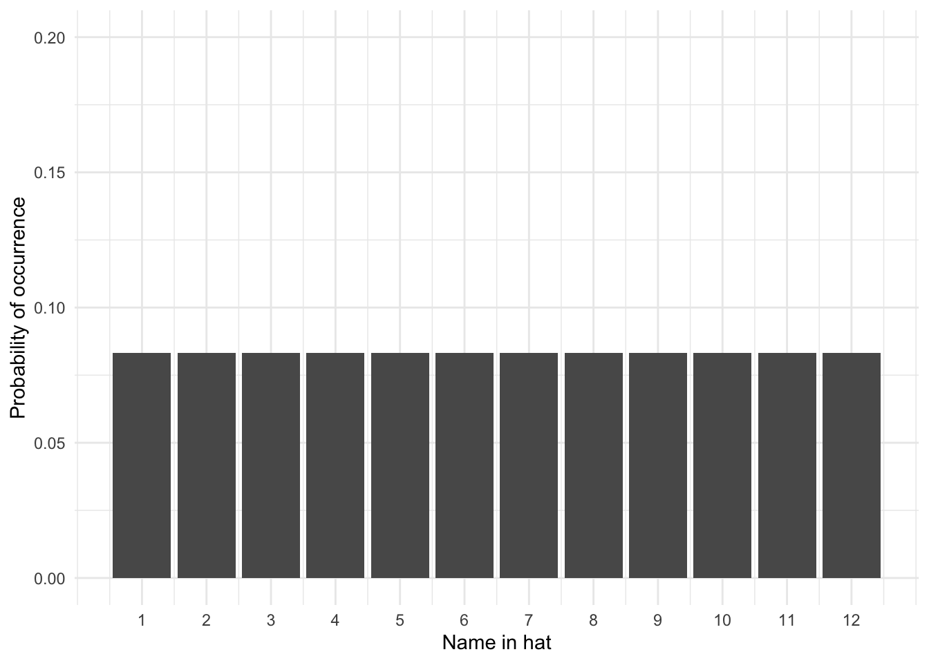
Figure 8.1: Uniform distribution
8.4.3 The binomial distribution
The binomial (bi = two, nominal = categories) distribution is a frequency distribution which calculates probabilities of success for situations where there are two possible outcomes e.g., flipping a coin. A binomial distribution models the probability of any number of successes being observed, given the probability of a success and the number of observations. Binomial distributions represent discrete data.
Describing the probability of single events, such as a single coin flip or rolling a six is easy, but more often than not we are interested in the probability of a collection of events, such as the number of heads out of 10 coin flips. To work this out, we can use the binomial distribution and functions in R.
Let’s say we flip a coin 10 times. Assuming the coin is fair (probability of heads = .5), how many heads should we expect to get? The below figure shows the results of a simulation for 10,000 coin flips (if you'd like to do this simulation yourself in R, you can see the code by clicking "Solution"). What this means is that we can use what we know about our data and the binomial distribution to work out the probability of different outcomes (e.g., what's the probability of getting at least 3 heads if you flip a coin 10 times?).
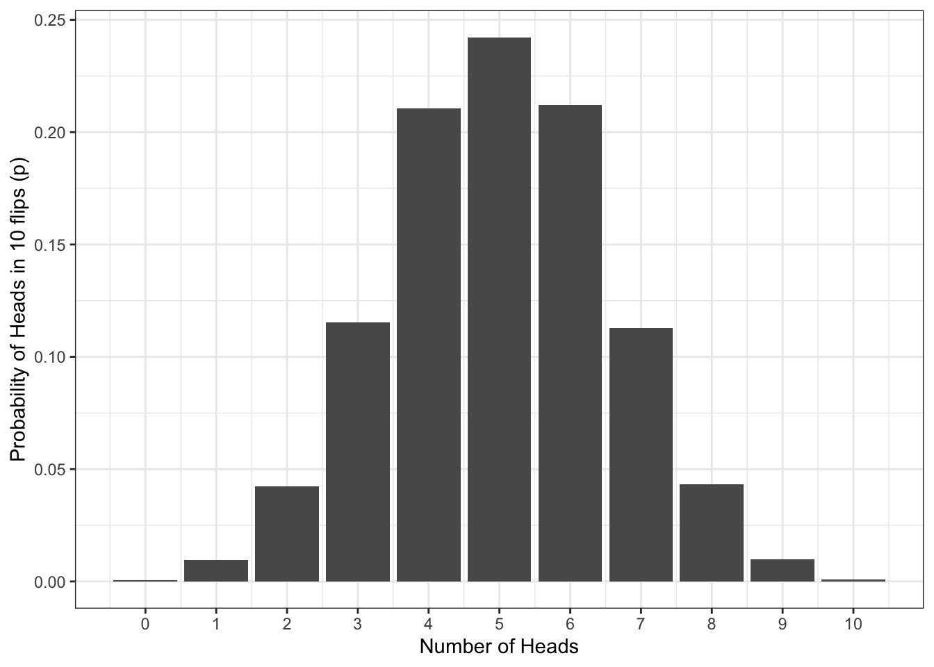
Figure 7.3: Probability of no. of heads from 10 coin tosses
heads10000 <- replicate(n = 10000, expr = sample(0:1, 10, TRUE) %>% sum())

data10000 <- tibble(heads = heads10000) %>%   # convert to a tibble
                group_by(heads) %>%     # group by number of possibilities
                summarise(n = n(), # count occurances of each possibility,
                          p=n/10000) # & calculate probability (p) of each

ggplot(data10000, aes(x = heads,y = p)) +
  geom_bar(stat = "identity") +
  labs(x = "Number of Heads", y = "Probability of Heads in 10 flips (p)") +
  theme_bw() +
  scale_x_continuous(breaks = c(0,1,2,3,4,5,6,7,8,9,10))
8.4.4 The normal distribution
The final probability distribution you need to know about is the normal distribution. The normal distribution, reflects the probability of any value occurring for a continuous variable. Examples of continuous variables include height or age, where a single person can score anywhere along a continuum. For example, a person could be 21.5 years old and 176cm tall.
As the normal distribution models the probability of a continuous variable, we plot the probability using a density plot. A normal distribution looks like this:

Figure 4.3: Normal Distribution of height. \(\mu\) = the mean (average), \(\sigma\) = standard deviation
Normal distributions are symmetrical, meaning there is an equal probability of observations occurring above and below the mean. This means that, if the mean in the below plot of heights is 170, we could expect the number of people who have a height of 160 to equal the number of people who have a height of 180. This also means that the mean, median, and mode are all expected to be equal in a normal distribution.
In the same way that we could with the coin flips, we can then use what we know about our data and the normal distribution to estimate the probability of certain outcomes (e.g., what's the probability that someone would be taller than 190cm?).
As with any probabilities, real-world data will come close to the normal distribution, but will (almost certainly) never match it exactly. As we collect more observations from normally-distributed data, our data will get increasingly closer to a normal distribution. As an example, here's a simulation of an experiment in which we collect heights from 5000 participants. As you can see, as we add more observations, our data starts to look more and more like the normal distribution in the previous figure.
Figure 7.4: A simulation of an experiment collecting height data from 2000 participants
8.5 Activity 3: Normal distribution
Complete the sentences so that they are correct.
- In a normal distribution, the mean, median, and mode .
- In a normal distribution, the further away from the mean an observation is .
- Whereas the binomial distribution is based on situations in which there are two possible outcomes, the normal distribution is based on situations in which the data .
8.6 Activity 4: Distribution test
Which distribution is likely to be associated with the following?
- Scores on an IQ test
- Whether a country has won or lost the Eurovision song contest
- Picking a spade card out of a normal pack of playing cards
8.7 Activity 5: Binomial distribution
Now, we're going to calculate probabilities based on the binomial distribution. In this chapter, for the first time we don't need to load the tidyverse. All of the functions we need are contained in Base R. If you want a refresher on the difference between Base R and packages, see Programming Basics.
- Open a new R Markdown document, call it "Probability" and save it in the relevant chapter folder.
We're going to use three Base R functions to work with the binomial distribution:
dbinom() - the density function: gives you the probability of x successes given the number of trials and the probability of success on a single trial (e.g., what's the probability of flipping 8/10 heads with a fair coin?).
pbinom() - the probability distribution function: gives you the cumulative probability of getting a number of successes below a certain cut-off point (e.g. probability of getting 0 to 5 heads out of 10 flips), given the size and the probability. This is known as the cumulative probability distribution function or the cumulative density function.
qbinom() - the quantile function: is the opposite of pbinom() in that it gives you the x axis value for a given probability p, plus given the size and prob, that is if the probability of flipping a head is .5, how many heads would you expect to get with 10 flips?
So let's try these functions out to answer two questions:
- What is the probability of getting exactly 5 heads on 10 flips?
- What is the probability of getting at most 2 heads on 10 flips?
8.8 Activity 6: dbinom()
Let's start with question 1, what is the probability of getting exactly 5 heads on 10 flips?
We want to predict the probability of getting 5 heads in 10 trials (coin flips) and the probability of success is 0.5 (it'll either be heads or tails so you have a 50/50 chance which we write as 0.5). We will use dbinom() to work this out:
The dbinom() (density) function has three arguments:
x: the number of ‘heads’ we want to know the probability of. Either a single one, 3 or a series 0:10. In this case it's 5.size: the number of trials (flips) we are simulating; in this case, 10 flips.prob: the probability of ‘heads’ on one trial. Here chance is 50-50 which as a probability we state as 0.5 or .5
Copy, paste and run the below code in a new code chunk:
dbinom(x = 5, size = 10, prob = 0.5)- What is the probability of getting 5 heads out of 10 coin flips to 2 decimal places?
- What is this probability expressed in percent?
8.9 Activity 7: pbinom()
OK, question number 2. What is the probability of getting at most 2 heads on 10 flips?
This time we use pbinom() as we want to know the cumulative probability of getting a maximum of 2 heads from 10 coin flips. so we have set a cut-off point of 2 but we still have a probability of getting a heads of 0.5.
Note: pbinom() takes the arguments size and prob argument just like dbinom(). However, the first input argument is q rather than x. This is because in dbinom x is a fixed number, whereas q is all the possibilities up to a given number (e.g. 0, 1, 2).
Copy, paste and run the below code in a new code chunk:
pbinom(q = 2, size = 10, prob = 0.5)- What is the probability of getting a maximum of 2 heads on 10 coin flips to 2 decimal places?
- What is this probability expressed in percent?
8.10 Activity 8: pbinom() 2
Let's try one more scenario with a cut-off point to make sure you have understood this. What is the probability of getting 7 or more heads on 10 flips?
We can use the same function as in the previous example, however, there's an extra argument if we want to get the correct answer. Let's try running the code we used above but change q = 2 to q = 7.
pbinom(q = 7, size = 10, prob = .5) ## [1] 0.9453125This tells us that the probability is .95 or 95% - that doesn't seem right does it? The default behaviour for pbinom() is to calculate cumulative probability for the lower tail of the curve, i.e., if you specify q = 2 it calculates the probability of all outcomes below 2. We specified q = 7 which means that it's calculated the probability of getting an outcome of 0, 1, 2, 3, 4, 5, 6, and 7, the blue area in the below figure - which is obviously very high.
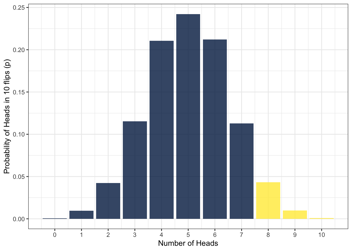
Figure 7.5: Lower and upper tails
To get the right answer, we have to add lower.tail = FALSE as we are interested in the upper tail of the distribution. Because we want the cumulative probability to include 7, we set q = 6. This will now calculate the cumulative probability of getting 7, 8, 9, or 10 heads out of 10 coin flips.
Copy, paste and run the below code in a new code chunk:
pbinom(q = 6, size = 10, prob = .5, lower.tail = FALSE) - What is the probability of getting between 7 and 10 heads from 10 coin flips to 2 decimal places?
- What is this probability expressed in percent?
8.11 Activity 9: qbinom()
OK, now let's consider a scenario in which you'd use the quantile function qbinom. Imagine that you've been accosted by a street magician and they want to bet you that they can predict whether the coin will land on heads or tails. You suspect that they've done something to the coin so that it's not fair and that the probability of the coin landing on a head is no longer .5 or 50/50, it's now more likely to land on tails. Your null hypothesis is that the coin is not dodgy and that the probability should be even (P(heads)=.5).You are going to run a single experiment to test your hypothesis, with 10 trials. What is the minimum number of heads that is acceptable if p really does equal .5?
You have used the argument prob in the previous two functions, dbinom and pbinom, and it represents the probability of success on a single trial (here it is the probability of 'heads' in one coin flip, .5). For qbinom, prob still represents the probability of success in one trial, whereas p represents the overall probability of success across all trials. When you run pbinom, it calculates the number of heads that would give that probability.
We know from looking at the binomial distribution above that sometimes even when the coin is fair, we won't get exactly 5/10 heads. Instead, we want to set a cut-off, a probability that below which well say that it's so unlikely we'd get that result if the coin was fair and in this example we will use the default cut-off for statistical significance in psychology, .05, or 5%.
In other words, you ask R for the minimum number of successes (e.g. heads) to maintain an overall probability of .05, in 10 flips, when the probability of a success on any one flip is .5.
qbinom(p = .05, size = 10, prob = .5)## [1] 2And it tells you the answer is 2. If the magician flipped fewer than two heads out of ten, you could conclude that there is a less than 5% probability that would happen if the coin was fair and you would reject the null hypothesis that the coin was unbiased against heads and tell the magician to do one.
qbinom also uses the lower.tail argument and it works in a similar fashion to pbinom.
However, ten trials is probably far too few if you want to accuse the magician of being a bit dodge. Run the below code and then answer the following questions:
- What would your cut-off be if you ran 100 trials?
- What would your cut-off be if you ran 1000 trials?
- What would your cut-off be if you ran 10,000 trials?
qbinom(p = .05, size = c(100, 1000, 10000), prob = .5)Notice that the more trials you run, the more precise the estimates become, that is, the closer they are to the probability of success on a single flip (.5). Again this is a simplification, but think about how this relates to sample size in research studies, the more participants you have, the more precise your estimate will be.
Visualise it!
Have a go at playing around with different numbers of coin flips and probabilities in our dbinom() and pbinom() app!
Figure 7.6: Binomial distribution app
8.12 Normal distribution
A similar set of functions exist to help us work with other distributions, including the normal distribution and we're going to use three of these:
dnorm()-the density function, for calculating the probability of a specific value
pnorm()-the probability or distribution function, for calculating the probability of getting at least or at most a specific value
qnorm()-the quantile function, for calculating the specific value associated with a given probability
As you can probably see, these functions are very similar to the functions we've already come across, that are used to work with the binomial distribution.
8.12.1 Probability of heights
Data from the Scottish Health Survey (2008) shows that:
- The average height of a 16-24 year old Scottish man is 176.2 centimetres, with a standard deviation of 6.748.
- The average height of a 16-24 year old Scottish woman is 163.8 cm, with a standard deviation of 6.931.
- There are currently no data on Scottish trans and non-binary people.
The below figure is a simulation of this data - you can see the code used to run this simulation by clicking the solution button.
men <- rnorm(n = 100000, mean = 176.2, sd = 6.748)
women <- rnorm(n = 100000, mean = 163.8, sd = 6.931)

heights <- tibble(men, women) %>%
  pivot_longer(names_to = "sex", values_to = "height", men:women)

ggplot(heights, aes(x = height, fill = sex)) +
  geom_density(alpha = .6) +
  scale_fill_viridis_d(option = "E") +
  theme_minimal()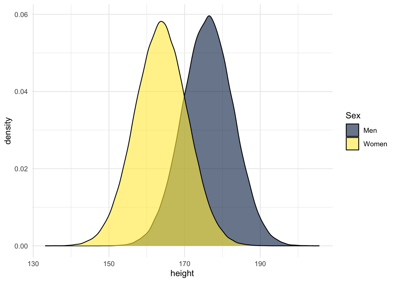
Figure 8.2: Simulation of Scottish height data
In this chapter we will use this information to calculate the probability of observing at least or at most a specific height with pnorm(), and the heights that are associated with specific probabilities with qnorm().
8.13 Activity 10:pnorm()
pnorm() requires three arguments:
qis the value that you want to calculate the probability ofmeanis the mean of the datasdis the standard deviation of the datalower.tailworks as above and depends on whether you are interested in the upper or lower tail
pnorm(q = NULL, mean = NULL, sd = NULL, lower.tail = NULL)Replace the NULLs in the above code to calculate the probability of meeting a 16-24 y.o. Scottish woman who is taller than the average 16-24 y.o. Scottish man.
- What is the probability of meeting a 16-24 y.o. Scottish woman who is taller than the average 16-24 y.o. Scottish man?
- What is this probability expressed in percent?
8.14 Activity 11: pnorm 2
Fiona is a very tall Scottish woman (181.12cm) in the 16-24 y.o. range who will only date men who are taller than her.
- Using
pnorm()again, what is the proportion of Scottish men Fiona would be willing to date to 2 decimal places?
- What is this probability expressed in percent?
8.15 Activity 12: pnorm 3
On the other hand, Fiona will only date women who are shorter than her.
- What is the proportion of Scottish women would Fiona be willing to date to 2 decimal places?
- What is this probability expressed in percent?
8.16 Activity 13: qnorm()
In the previous examples we calculated the probability of a particular outcome. Now we want to calculate what outcome would be associated with a particular probability and we can use qnorm() to do this.
qnorm() is very similar to pnorm() with one exception, rather than specifying q our known observation or quantile, instead we have to specify p, our known probability.
qnorm(p = NULL, mean = NULL, sd = NULL, lower.tail = NULL)Replace the NULLs in the above code to calculate how tall a 16-24 y.o. Scottish man would have to be in order to be in the top 5% (i.e., p = .05) of the height distribution for Scottish men in his age group.
Visualise it!
Have a go at playing around with different distributions in our dnorm() and pnorm() app - access it here
And that's it! The key concepts to take away from this chapter are that different types of data tend to follow known distributions, and that we can use these distributions to calculate the probability of particular outcomes. This is the foundation of many of the statistical tests that you will learn about in this course.
For example, if you want to compare whether the scores from two groups are different, that is, whether they come from different distributions, you can calculate the probability that the scores from group 2 would be in the same distribution as group 1. If this probability is less than 5% (p = .05), you might conclude that the scores were significantly different. That's an oversimplification obviously, but if you can develop a good understanding of probability distributions it will stand you in good stead for the rest of the statistics content.
8.17 Activity solutions
8.17.1 Activity 6
.258.17.2 Activity 7
.068.17.3 Activity 8
.178.17.4 Activity 10
pnorm(q = 176.2, mean = 163.8, sd = 6.931, lower.tail = FALSE)8.17.5 Activity 11
pnorm(q = 181.12, mean = 176.2, sd = 6.748, lower.tail = FALSE)8.17.6 Activity 12
pnorm(q = 181.12, mean = 163.8, sd = 6.931, lower.tail = TRUE)8.17.7 Activity 13
qnorm(p = .05, mean = 176.2, sd = 6.748, lower.tail = FALSE)