Chapter 10 Reproducible Workflows
10.1 Learning Objectives
10.1.1 Basic
- Create a reproducible script in R Markdown
- Edit the YAML header to add table of contents and other options
- Include a table
- Include a figure
- Use
source()to include code from an external file - Report the output of an analysis using inline R
10.1.2 Intermediate
- Output doc and PDF formats
- Add a bibliography and in-line citations
- Format tables using
kableExtra
10.1.3 Advanced
- Create a computationally reproducible project in Code Ocean
10.2 Resources
- Chapter 27: R Markdown in R for Data Science
- R Markdown Cheat Sheet
- R Markdown reference Guide
- R Markdown Tutorial
- R Markdown: The Definitive Guide by Yihui Xie, J. J. Allaire, & Garrett Grolemund
- Papaja Reproducible APA Manuscripts
- Code Ocean for Computational Reproducibility
10.3 Setup
library(tidyverse)
library(knitr)
library(broom)
set.seed(8675309)
10.4 R Markdown
By now you should be pretty comfortable working with R Markdown files from the weekly formative exercises and set exercises. Here, we’ll explore some of the more advanced options and create an R Markdown document that produces a reproducible manuscript.
First, make a new R Markdown document.
10.4.1 knitr options
When you create a new R Markdown file in RStudio, a setup chunk is automatically created.
```{r setup, include=FALSE}
knitr::opts_chunk$set(echo = TRUE)```
You can set more default options for code chunks here. See the knitr options documentation for explanations of the possible options.
```{r setup, include=FALSE}
knitr::opts_chunk$set(
  fig.width  = 8,
  fig.height = 5,
  fig.path   = 'images/',
  echo       = FALSE,
  warning    = TRUE,
  message    = FALSE,
  cache      = FALSE
)
```
The code above sets the following options:
fig.width = 8: figure width is 8 inchesfig.height = 5: figure height is 5 inchesfig.path = 'images/': figures are saved in the directory “images”echo = FALSE: do not show code chunks in the rendered documentwarning = FALSE: do not show any function warningsmessage = FALSE: do not show any function messagescache = FALSE: run all the code to create all of the images and objects each time you knit (set toTRUEif you have time-consuming code)
10.4.2 YAML Header
The YAML header is where you can set several options.
---
title: "My Demo Document"
author: "Me"
output:
  html_document:
    theme: spacelab
    highlight: tango
    toc: true
    toc_float:
      collapsed: false
      smooth_scroll: false
    toc_depth: 3
    number_sections: false
---
The built-in themes are: “cerulean,” “cosmo,” “flatly,” “journal,” “lumen,” “paper,” “readable,” “sandstone,” “simplex,” “spacelab,” “united,” and “yeti.” You can view and download more themes.
Try changing the values from false to true to see what the options do.
10.4.3 TOC and Document Headers
If you include a table of contents (toc), it is created from your document headers. Headers in markdown are created by prefacing the header title with one or more hashes (#). Add a typical paper structure to your document like the one below.
## Abstract

My abstract here...

## Introduction

What's the question; why is it interesting?

## Methods

### Participants

How many participants and why? Do your power calculation here.

### Procedure

What will they do?

### Analysis

Describe the analysis plan...

## Results

Demo results for simulated data...

## Discussion

What does it all mean?

## References
10.4.4 Code Chunks
You can include code chunks that create and display images, tables, or computations to include in your text. Let’s start by simulating some data.
First, create a code chunk in your document. You can put this before the abstract, since we won’t be showing the code in this document. We’ll use a modified version of the two_sample function from the GLM lecture to create two groups with a difference of 0.75 and 100 observations per group.
This function was modified to add sex and effect-code both sex and group. Using the recode function to set effect or difference coding makes it clearer which value corresponds to which level. There is no effect of sex or interaction with group in these simulated data.
two_sample <- function(diff = 0.5, n_per_group = 20) {
  tibble(Y = c(rnorm(n_per_group, -.5 * diff, sd = 1),
               rnorm(n_per_group, .5 * diff, sd = 1)),
         grp = factor(rep(c("a", "b"), each = n_per_group)),
         sex = factor(rep(c("female", "male"), times = n_per_group))
  ) %>%
    mutate(
      grp_e = recode(grp, "a" = -0.5, "b" = 0.5),
      sex_e = recode(sex, "female" = -0.5, "male" = 0.5)
    )
}
This function requires the tibble and dplyr packages, so remember to load the whole tidyverse package at the top of this script (e.g., in the setup chunk).
Now we can make a separate code chunk to create our simulated dataset dat.
dat <- two_sample(diff = 0.75, n_per_group = 100)10.4.4.1 Tables
Next, create a code chunk where you want to display a table of the descriptives (e.g., Participants section of the Methods). We’ll use tidyverse functions you learned in the data wrangling lectures to create summary statistics for each group.
```{r, results='asis'}

dat %>%
  group_by(grp, sex) %>%
  summarise(n = n(),
            Mean = mean(Y),
            SD = sd(Y)) %>%
  rename(group = grp) %>%
  mutate_if(is.numeric, round, 3) %>%
  knitr::kable()

```
## `summarise()` has grouped output by 'grp'. You can override using the `.groups` argument.## `mutate_if()` ignored the following grouping variables:
## Column `group`| group | sex | n | Mean | SD |
|---|---|---|---|---|
| a | female | 50 | -0.361 | 0.796 |
| a | male | 50 | -0.284 | 1.052 |
| b | female | 50 | 0.335 | 1.080 |
| b | male | 50 | 0.313 | 0.904 |
Notice that the r chunk specifies the option results='asis'. This lets you format the table using the kable() function from knitr. You can also use more specialised functions from papaja or kableExtra to format your tables.
10.4.4.2 Images
Next, create a code chunk where you want to display the image in your document. Let’s put it in the Results section. Use what you learned in the data visualisation lecture to show violin-boxplots for the two groups.
```{r, fig1, fig.cap="Figure 1. Scores by group and sex."}
ggplot(dat, aes(grp, Y, fill = sex)) +
  geom_violin(alpha = 0.5) +
  geom_boxplot(width = 0.25,
               position = position_dodge(width = 0.9),
               show.legend = FALSE) +
  scale_fill_manual(values = c("orange", "purple")) +
  xlab("Group") +
  ylab("Score") +
  theme(text = element_text(size = 30, family = "Times"))

```
The last line changes the default text size and font, which can be useful for generating figures that meet a journal’s requirements.
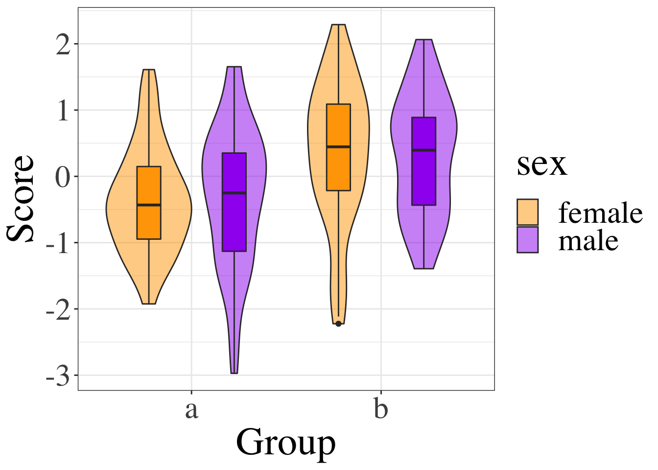
Figure 10.1: Figure 1. Scores by group and sex.
You can also include images that you did not create in R using the typical markdown syntax for images:
](images/memes/x-all-the-things.png)
All the Things by Hyperbole and a Half
10.4.4.3 In-line R
Now let’s use what you learned in the GLM lecture to analyse our simulated data. The document is getting a little cluttered, so let’s move this code to external scripts.
- Create a new R script called “functions.R”
- Move the
library(tidyverse)line and thetwo_sample()function definition to this file. - Create a new R script called “analysis.R”
- Move the code for creating
datto this file. - Add the following code to the end of the setup chunk:
source("functions.R")
source("analysis.R")
The source function lets you include code from an external file. This is really useful for making your documents readable. Just make sure you call your source files in the right order (e.g., include function definitions before you use the functions).
In the “analysis.R” file, we’re going to run the analysis code and save any numbers we might want to use in our manuscript to variables.
grp_lm <- lm(Y ~ grp_e * sex_e, data = dat)

stats <- grp_lm %>%
  broom::tidy() %>%
  mutate_if(is.numeric, round, 3)
The code above runs our analysis predicting Y from the effect-coded group variable grp_e, the effect-coded sex variable sex_e and their intereaction. The tidy function from the broom package turns the output into a tidy table. The mutate_if function uses the function is.numeric to check if each column should be mutated, adn if it is numeric, applies the round function with the digits argument set to 3.
If you want to report the results of the analysis in a paragraph istead of a table, you need to know how to refer to each number in the table. Like with everything in R, there are many wways to do this. One is by specifying the column and row number like this:
stats$p.value[2]## [1] 0Another way is to create variables for each row like this:
grp_stats <- filter(stats, term == "grp_e")
sex_stats <- filter(stats, term == "sex_e")
ixn_stats <- filter(stats, term == "grp_e:sex_e")
Add the above code to the end of your analysis.R file. Then you can refer to columns by name like this:
grp_stats$p.value
sex_stats$statistic
ixn_stats$estimate
## [1] 0
## [1] 0.197
## [1] -0.099You can insert these numbers into a paragraph with inline R code that looks like this:
Scores were higher in group B than group A
(B = `r grp_stats$estimate`,
t = `r grp_stats$statistic`,
p = `r grp_stats$p.value`).
There was no significant difference between men and women
(B = `r sex_statsestimate`,
t = `r sex_stats$statistic`,
p = `r sex_stats$p.value`)
and the effect of group was not qualified by an interaction with sex
(B = `r ixn_stats$estimate`,
t = `r ixn_stats$statistic`,
p = `r ixn_stats$p.value`).
Rendered text:
Scores were higher in group B than group A
(B = 0.647,
t = 4.74,
p = 0).
There was no significant difference between men and women
(B = 0.027,
t = 0.197,
p = 0.844)
and the effect of group was not qualified by an interaction with sex
(B = -0.099,
t = -0.363,
p = 0.717).
Remember, line breaks are ignored when you render the file (unless you add two spaces at the end of lines), so you can use line breaks to make it easier to read your text with inline R code.
The p-values aren’t formatted in APA style. We wrote a function to deal with this in the function lecture. Add this function to the “functions.R” file and change the inline text to use the report_p function.
report_p <- function(p, digits = 3) {
  if (!is.numeric(p)) stop("p must be a number")
  if (p <= 0) warning("p-values are normally greater than 0")
  if (p >= 1) warning("p-values are normally less than 1")

  if (p < .001) {
    reported = "p < .001"
  } else {
    roundp <- round(p, digits)
    fmt <- paste0("p = %.", digits, "f")
    reported = sprintf(fmt, roundp)
  }

  reported
}
Scores were higher in group B than group A
(B = `r grp_stats$estimate`,
t = `r grp_stats$statistic`,
`r report_p(grp_stats$p.value, 3)`).
There was no significant difference between men and women
(B = `r sex_stats$estimate`,
t = `r sex_stats$statistic`,
`r report_p(sex_stats$p.value, 3)`)
and the effect of group was not qualified by an interaction with sex
(B = `r ixn_stats$estimate`,
t = `r ixn_stats$statistic`,
`r report_p(ixn_stats$p.value, 3)`).
Rendered text:
Scores were higher in group B than group A
(B = 0.647,
t = 4.74,
p < .001).
There was no significant difference between men and women
(B = 0.027,
t = 0.197,
p = 0.844)
and the effect of group was not qualified by an interaction with sex
(B = -0.099,
t = -0.363,
p = 0.717).
You might also want to report the statistics for the regression. There are a lot of numbers to format and insert, so it is easier to do this in the analysis script using sprintf for formatting.
s <- summary(grp_lm)

# calculate p value from fstatistic
fstat.p <- pf(s$fstatistic[1],
              s$fstatistic[2],
              s$fstatistic[3],
              lower=FALSE)

adj_r <- sprintf(
  "The regression equation had an adjusted $R^{2}$ of %.3f ($F_{(%i, %i)}$ = %.3f, %s).",
  round(s$adj.r.squared, 3),
  s$fstatistic[2],
  s$fstatistic[3],
  round(s$fstatistic[1], 3),
  report_p(fstat.p, 3)
)
Then you can just insert the text in your manuscript like this: ` adj_r`:
The regression equation had an adjusted \(R^{2}\) of 0.090 (\(F_{(3, 196)}\) = 7.546, p < .001).
10.4.5 Bibliography
There are several ways to do in-text citations and automatically generate a bibliography in RMarkdown.
10.4.5.1 Create a BibTeX File Manually
You can just make a BibTeX file and add citations manually. Make a new Text File in RStudio called “bibliography.bib.”
Next, add the line bibliography: bibliography.bib to your YAML header.
You can add citations in the following format:
@article{shortname,
  author = {Author One and Author Two and Author Three},
  title = {Paper Title},
  journal = {Journal Title},
  volume = {vol},
  number = {issue},
  pages = {startpage--endpage},
  year = {year},
  doi = {doi}
}
10.4.5.2 Citing R packages
You can get the citation for an R package using the function citation. You can paste the bibtex entry into your bibliography.bib file. Make sure to add a short name (e.g., “rmarkdown”) before the first comma to refer to the reference.
citation(package="rmarkdown")##
## To cite the 'rmarkdown' package in publications, please use:
##
## JJ Allaire and Yihui Xie and Jonathan McPherson and Javier Luraschi
## and Kevin Ushey and Aron Atkins and Hadley Wickham and Joe Cheng and
## Winston Chang and Richard Iannone (2021). rmarkdown: Dynamic
## Documents for R. R package version 2.9.4. URL
## https://rmarkdown.rstudio.com.
##
## Yihui Xie and J.J. Allaire and Garrett Grolemund (2018). R Markdown:
## The Definitive Guide. Chapman and Hall/CRC. ISBN 9781138359338. URL
## https://bookdown.org/yihui/rmarkdown.
##
## Yihui Xie and Christophe Dervieux and Emily Riederer (2020). R
## Markdown Cookbook. Chapman and Hall/CRC. ISBN 9780367563837. URL
## https://bookdown.org/yihui/rmarkdown-cookbook.
##
## To see these entries in BibTeX format, use 'print(<citation>,
## bibtex=TRUE)', 'toBibtex(.)', or set
## 'options(citation.bibtex.max=999)'.10.4.5.3 Download Citation Info
You can get the BibTeX formatted citation from most publisher websites. For example, go to the publisher’s page for Equivalence Testing for Psychological Research: A Tutorial, click on the Cite button (in the sidebar or under the bottom Explore More menu), choose BibTeX format, and download the citation. You can open up the file in a text editor and copy the text. It should look like this:
@article{doi:10.1177/2515245918770963,
author = {Daniël Lakens and Anne M. Scheel and Peder M. Isager},
title ={Equivalence Testing for Psychological Research: A Tutorial},
journal = {Advances in Methods and Practices in Psychological Science},
volume = {1},
number = {2},
pages = {259-269},
year = {2018},
doi = {10.1177/2515245918770963},

URL = {
        https://doi.org/10.1177/2515245918770963

},
eprint = {
        https://doi.org/10.1177/2515245918770963

}
,
    abstract = { Psychologists must be able to test both for the presence of an effect and for the absence of an effect. In addition to testing against zero, researchers can use the two one-sided tests (TOST) procedure to test for equivalence and reject the presence of a smallest effect size of interest (SESOI). The TOST procedure can be used to determine if an observed effect is surprisingly small, given that a true effect at least as extreme as the SESOI exists. We explain a range of approaches to determine the SESOI in psychological science and provide detailed examples of how equivalence tests should be performed and reported. Equivalence tests are an important extension of the statistical tools psychologists currently use and enable researchers to falsify predictions about the presence, and declare the absence, of meaningful effects. }
}
Paste the reference into your bibliography.bib file. Change doi:10.1177/2515245918770963 in the first line of the reference to a short string you will use to cite the reference in your manuscript. We’ll use TOSTtutorial.
10.4.5.4 Converting from reference software
Most reference software like EndNote, Zotero or mendeley have exporting options that can export to BibTeX format. You just need to check the shortnames in the resulting file.
10.4.5.5 In-text citations
You can cite reference in text like this:
This tutorial uses several R packages [@tidyverse;@rmarkdown].This tutorial uses several R packages (Wickham 2017; Allaire et al. 2018).
Put a minus in front of the @ if you just want the year:
Lakens, Scheel and Isengar [-@TOSTtutorial] wrote a tutorial explaining how to test for the absence of an effect.Lakens, Scheel and Isengar (2018) wrote a tutorial explaining how to test for the absence of an effect.
10.4.5.6 Citation Styles
You can search a list of style files for various journals and download a file that will format your bibliography for a specific journal’s style. You’ll need to add the line csl: filename.csl to your YAML header.
Add some citations to your bibliography.bib file, reference them in your text, and render your manuscript to see the automatically generated reference section. Try a few different citation style files.
10.4.6 Output Formats
You can knit your file to PDF or Word if you have the right packages installed on your computer.
10.4.7 Computational Reproducibility
Computational reproducibility refers to making all aspects of your analysis reproducible, including specifics of the software you used to run the code you wrote. R packages get updated periodically and some of these updates may break your code. Using a computational reproducibility platform guards against this by always running your code in the same environment.
Code Ocean is a new platform that lets you run your code in the cloud via a web browser.
10.5 Glossary
| term | definition |
|---|---|
| chunk | A section of code in an R Markdown file |
| markdown | A way to specify formatting, such as headers, paragraphs, lists, bolding, and links. |
| reproducibility | The extent to which the findings of a study can be repeated in some other context |
| yaml | A structured format for information |