Chapter 2 Working with Data
2.1 Learning Objectives
- Load built-in datasets (video)
- Import data from CSV and Excel files (video)
- Create a data table (video)
- Understand the use the basic data types (video)
- Understand and use the basic container types (list, vector) (video)
- Use vectorized operations (video)
- Be able to troubleshoot common data import problems (video)
2.2 Resources
2.3 Setup
# libraries needed for these examples
library(tidyverse)
library(dataskills)
2.4 Data tables
2.4.1 Built-in data
R comes with built-in datasets. Some packages, like tidyr and dataskills, also contain data. The data() function lists the datasets available in a package.
# lists datasets in dataskills
data(package = "dataskills")
Type the name of a dataset into the console to see the data. Type ?smalldata into the console to see the dataset description.
smalldata| id | group | pre | post |
|---|---|---|---|
| S01 | control | 98.46606 | 106.70508 |
| S02 | control | 104.39774 | 89.09030 |
| S03 | control | 105.13377 | 123.67230 |
| S04 | control | 92.42574 | 70.70178 |
| S05 | control | 123.53268 | 124.95526 |
| S06 | exp | 97.48676 | 101.61697 |
| S07 | exp | 87.75594 | 126.30077 |
| S08 | exp | 77.15375 | 72.31229 |
| S09 | exp | 97.00283 | 108.80713 |
| S10 | exp | 102.32338 | 113.74732 |
You can also use the data() function to load a dataset into your global environment.
# loads smalldata into the environment
data("smalldata")
Always, always, always, look at your data once you’ve created or loaded a table. Also look at it after each step that transforms your table. There are three main ways to look at your tibble: print(), glimpse(), and View().
The print() method can be run explicitly, but is more commonly called by just typing the variable name on the blank line. The default is not to print the entire table, but just the first 10 rows. It’s rare to print your data in a script; that is something you usually are doing for a sanity check, and you should just do it in the console.
Let’s look at the smalldata table that we made above.
smalldata| id | group | pre | post |
|---|---|---|---|
| S01 | control | 98.46606 | 106.70508 |
| S02 | control | 104.39774 | 89.09030 |
| S03 | control | 105.13377 | 123.67230 |
| S04 | control | 92.42574 | 70.70178 |
| S05 | control | 123.53268 | 124.95526 |
| S06 | exp | 97.48676 | 101.61697 |
| S07 | exp | 87.75594 | 126.30077 |
| S08 | exp | 77.15375 | 72.31229 |
| S09 | exp | 97.00283 | 108.80713 |
| S10 | exp | 102.32338 | 113.74732 |
The function glimpse() gives a sideways version of the tibble. This is useful if the table is very wide and you can’t see all of the columns. It also tells you the data type of each column in angled brackets after each column name. We’ll learn about data types below.
glimpse(smalldata)## Rows: 10
## Columns: 4
## $ id <chr> "S01", "S02", "S03", "S04", "S05", "S06", "S07", "S08", "S09", "…
## $ group <chr> "control", "control", "control", "control", "control", "exp", "e…
## $ pre <dbl> 98.46606, 104.39774, 105.13377, 92.42574, 123.53268, 97.48676, 8…
## $ post <dbl> 106.70508, 89.09030, 123.67230, 70.70178, 124.95526, 101.61697, …The other way to look at the table is a more graphical spreadsheet-like version given by View() (capital ‘V’). It can be useful in the console, but don’t ever put this one in a script because it will create an annoying pop-up window when the user runs it.
Now you can click on smalldata in the environment pane to open it up in a viewer that looks a bit like Excel.
You can get a quick summary of a dataset with the summary() function.
summary(smalldata)## id group pre post
## Length:10 Length:10 Min. : 77.15 Min. : 70.70
## Class :character Class :character 1st Qu.: 93.57 1st Qu.: 92.22
## Mode :character Mode :character Median : 97.98 Median :107.76
## Mean : 98.57 Mean :103.79
## 3rd Qu.:103.88 3rd Qu.:121.19
## Max. :123.53 Max. :126.30You can even do things like calculate the difference between the means of two columns.
pre_mean <- mean(smalldata$pre)
post_mean <- mean(smalldata$post)
post_mean - pre_mean
## [1] 5.2230552.4.2 Importing data
Built-in data are nice for examples, but you’re probably more interested in your own data. There are many different types of files that you might work with when doing data analysis. These different file types are usually distinguished by the three letter extension following a period at the end of the file name. Here are some examples of different types of files and the functions you would use to read them in or write them out.
| Extension | File Type | Reading | Writing |
|---|---|---|---|
| .csv | Comma-separated values | readr::read_csv() |
readr::write_csv() |
| .tsv, .txt | Tab-separated values | readr::read_tsv() |
readr::write_tsv() |
| .xls, .xlsx | Excel workbook | readxl::read_excel() |
NA |
| .sav, .mat, … | Multiple types | rio::import() |
NA |
The double colon means that the function on the right comes from the package on the left, so readr::read_csv() refers to the read_csv() function in the readr package, and readxl::read_excel() refers to the function read_excel() in the package readxl. The function rio::import() from the rio package will read almost any type of data file, including SPSS and Matlab. Check the help with ?rio::import to see a full list.
You can get a directory of data files used in this class for tutorials and exercises with the following code, which will create a directory called “data” in your project directory. Alternatively, you can download a zip file of the datasets.
dataskills::getdata()Probably the most common file type you will encounter is .csv (comma-separated values). As the name suggests, a CSV file distinguishes which values go with which variable by separating them with commas, and text values are sometimes enclosed in double quotes. The first line of a file usually provides the names of the variables.
For example, here are the first few lines of a CSV containing personality scores:
  subj_id,O,C,E,A,N
  S01,4.428571429,4.5,3.333333333,5.142857143,1.625
  S02,5.714285714,2.9,3.222222222,3,2.625
  S03,5.142857143,2.8,6,3.571428571,2.5
  S04,3.142857143,5.2,1.333333333,1.571428571,3.125
  S05,5.428571429,4.4,2.444444444,4.714285714,1.625
  ```

There are six variables in this dataset, and their names are given in the first line of the file: `subj_id`, `O`, `C`, `E`, `A`, and `N`. You can see that the values for each of these variables are given in order, separated by commas, on each subsequent line of the file.

When you read in CSV files, it is best practice to use the `readr::read_csv()` function. The `readr` package is automatically loaded as part of the `tidyverse` package, which we will be using in almost every script. Note that you would normally want to store the result of the `read_csv()` function to an object, as so:


```r
csv_data <- read_csv("data/5factor.csv")
##
## ── Column specification ────────────────────────────────────────────────────────
## cols(
## subj_id = col_character(),
## O = col_double(),
## C = col_double(),
## E = col_double(),
## A = col_double(),
## N = col_double()
## )The read_csv() and read_tsv() functions will give you some information about the data you just read in so you can check the column names and data types. For now, it’s enough to know that col_double() refers to columns with numbers and col_character() refers to columns with words. We’ll learn in the toroubleshooting section below how to fix it if the function guesses the wrong data type.
tsv_data <- read_tsv("data/5factor.txt")
xls_data <- readxl::read_xls("data/5factor.xls")
# you can load sheets from excel files by name or number
rep_data <- readxl::read_xls("data/5factor.xls", sheet = "replication")
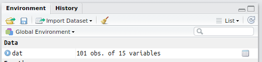
spss_data <- rio::import("data/5factor.sav")Once loaded, you can view your data using the data viewer. In the upper right hand window of RStudio, under the Environment tab, you will see the object babynames listed.
If you click on the View icon (![]() ), it will bring up a table view of the data you loaded in the top left pane of RStudio.
), it will bring up a table view of the data you loaded in the top left pane of RStudio.

This allows you to check that the data have been loaded in properly. You can close the tab when you’re done looking at it, it won’t remove the object.
2.4.3 Creating data
If we are creating a data table from scratch, we can use the tibble::tibble() function, and type the data right in. The tibble package is part of the tidyverse package that we loaded at the start of this chapter.
Let’s create a small table with the names of three Avatar characters and their bending type. The tibble() function takes arguments with the names that you want your columns to have. The values are vectors that list the column values in order.
If you don’t know the value for one of the cells, you can enter NA, which we have to do for Sokka because he doesn’t have any bending ability. If all the values in the column are the same, you can just enter one value and it will be copied for each row.
avatar <- tibble(
  name = c("Katara", "Toph", "Sokka"),
  bends = c("water", "earth", NA),
  friendly = TRUE
)

# print it
avatar| name | bends | friendly |
|---|---|---|
| Katara | water | TRUE |
| Toph | earth | TRUE |
| Sokka | NA | TRUE |
2.4.4 Writing Data
If you have data that you want to save to a CSV file, use readr::write_csv(), as follows.
write_csv(avatar, "avatar.csv")This will save the data in CSV format to your working directory.
-
Create a new table called
familywith the first name, last name, and age of your family members. - Save it to a CSV file called “family.csv.”
-
Clear the object from your environment by restarting R or with the code
remove(family). - Load the data back in and view it.
We’ll be working with tabular data a lot in this class, but tabular data is made up of vectors, which group together data with the same basic data type. The following sections explain some of this terminology to help you understand the functions we’ll be learning to process and analyse data.
2.5 Basic data types
Data can be numbers, words, true/false values or combinations of these. In order to understand some later concepts, it’s useful to have a basic understanding of data types in R: numeric, character, and logical There is also a specific data type called a factor, which will probably give you a headache sooner or later, but we can ignore it for now.
2.5.1 Numeric data
All of the real numbers are numeric data types (imaginary numbers are “complex”). There are two types of numeric data, integer and double. Integers are the whole numbers, like -1, 0 and 1. Doubles are numbers that can have fractional amounts. If you just type a plain number such as 10, it is stored as a double, even if it doesn’t have a decimal point. If you want it to be an exact integer, use the L suffix (10L).
If you ever want to know the data type of something, use the typeof function.
typeof(10)   # double
typeof(10.0) # double
typeof(10L)  # integer
typeof(10i)  # complex
## [1] "double"
## [1] "double"
## [1] "integer"
## [1] "complex"If you want to know if something is numeric (a double or an integer), you can use the function is.numeric() and it will tell you if it is numeric (TRUE) or not (FALSE).
is.numeric(10L)
is.numeric(10.0)
is.numeric("Not a number")
## [1] TRUE
## [1] TRUE
## [1] FALSE2.5.2 Character data
Character strings are any text between quotation marks.
typeof("This is a character string")
typeof('You can use double or single quotes')
## [1] "character"
## [1] "character"This can include quotes, but you have to escape it using a backslash to signal the the quote isn’t meant to be the end of the string.
my_string <- "The instructor said, \"R is cool,\" and the class agreed."
cat(my_string) # cat() prints the arguments
## The instructor said, "R is cool," and the class agreed.2.5.3 Logical Data
Logical data (also sometimes called “boolean” values) is one of two values: true or false. In R, we always write them in uppercase: TRUE and FALSE.
class(TRUE)
class(FALSE)
## [1] "logical"
## [1] "logical"When you compare two values with an operator, such as checking to see if 10 is greater than 5, the resulting value is logical.
is.logical(10 > 5)## [1] TRUE
You might also see logical values abbreviated as T and F, or 0 and 1. This can cause some problems down the road, so we will always spell out the whole thing.
What data types are these:
100100L"100"100.0-100Lfactor(100)TRUE"TRUE"FALSE1 == 2
2.6 Basic container types
Individual data values can be grouped together into containers. The main types of containers we’ll work with are vectors, lists, and data tables.
2.6.1 Vectors
A vector in R is like a vector in mathematics: a set of ordered elements. All of the elements in a vector must be of the same data type (numeric, character, logical). You can create a vector by enclosing the elements in the function c().
## put information into a vector using c(...)
c(1, 2, 3, 4)
c("this", "is", "cool")
1:6 # shortcut to make a vector of all integers x:y
## [1] 1 2 3 4
## [1] "this" "is" "cool"
## [1] 1 2 3 4 5 6What happens when you mix types? What class is the variable mixed?
mixed <- c(2, "good", 2L, "b", TRUE)
You can’t mix data types in a vector; all elements of the vector must be the same data type. If you mix them, R will “coerce” them so that they are all the same. If you mix doubles and integers, the integers will be changed to doubles. If you mix characters and numeric types, the numbers will be coerced to characters, so 10 would turn into “10.”
2.6.1.1 Selecting values from a vector
If we wanted to pick specific values out of a vector by position, we can use square brackets (an extract operator, or []) after the vector.
values <- c(10, 20, 30, 40, 50)
values[2] # selects the second value
## [1] 20You can select more than one value from the vector by putting a vector of numbers inside the square brackets. For example, you can select the 18th, 19th, 20th, 21st, 4th, 9th and 15th letter from the built-in vector LETTERS (which gives all the uppercase letters in the Latin alphabet).
word <- c(18, 19, 20, 21, 4, 9, 15)
LETTERS[word]
## [1] "R" "S" "T" "U" "D" "I" "O"Can you decode the secret message?
secret <- c(14, 5, 22, 5, 18, 7, 15, 14, 14, 1, 7, 9, 22, 5, 25, 15, 21, 21, 16)You can also create ‘named’ vectors, where each element has a name. For example:
vec <- c(first = 77.9, second = -13.2, third = 100.1)
vec
## first second third
## 77.9 -13.2 100.1We can then access elements by name using a character vector within the square brackets. We can put them in any order we want, and we can repeat elements:
vec[c("third", "second", "second")]## third second second
## 100.1 -13.2 -13.2
We can get the vector of names using the names() function, and we can set or change them using something like names(vec2) <- c(“n1,” “n2,” “n3”).
Another way to access elements is by using a logical vector within the square brackets. This will pull out the elements of the vector for which the corresponding element of the logical vector is TRUE. If the logical vector doesn’t have the same length as the original, it will repeat. You can find out how long a vector is using the length() function.
length(LETTERS)
LETTERS[c(TRUE, FALSE)]
## [1] 26
## [1] "A" "C" "E" "G" "I" "K" "M" "O" "Q" "S" "U" "W" "Y"2.6.1.2 Repeating Sequences
Here are some useful tricks to save typing when creating vectors.
In the command x:y the : operator would give you the sequence of number starting at x, and going to y in increments of 1.
1:10
15.3:20.5
0:-10
## [1] 1 2 3 4 5 6 7 8 9 10
## [1] 15.3 16.3 17.3 18.3 19.3 20.3
## [1] 0 -1 -2 -3 -4 -5 -6 -7 -8 -9 -10What if you want to create a sequence but with something other than integer steps? You can use the seq() function. Look at the examples below and work out what the arguments do.
seq(from = -1, to = 1, by = 0.2)
seq(0, 100, length.out = 11)
seq(0, 10, along.with = LETTERS)
## [1] -1.0 -0.8 -0.6 -0.4 -0.2 0.0 0.2 0.4 0.6 0.8 1.0
## [1] 0 10 20 30 40 50 60 70 80 90 100
## [1] 0.0 0.4 0.8 1.2 1.6 2.0 2.4 2.8 3.2 3.6 4.0 4.4 4.8 5.2 5.6
## [16] 6.0 6.4 6.8 7.2 7.6 8.0 8.4 8.8 9.2 9.6 10.0What if you want to repeat a vector many times? You could either type it out (painful) or use the rep() function, which can repeat vectors in different ways.
rep(0, 10)                      # ten zeroes
rep(c(1L, 3L), times = 7)       # alternating 1 and 3, 7 times
rep(c("A", "B", "C"), each = 2) # A to C, 2 times each
## [1] 0 0 0 0 0 0 0 0 0 0
## [1] 1 3 1 3 1 3 1 3 1 3 1 3 1 3
## [1] "A" "A" "B" "B" "C" "C"The rep() function is useful to create a vector of logical values (TRUE/FALSE or 1/0) to select values from another vector.
# Get subject IDs in the pattern Y Y N N ...
subject_ids <- 1:40
yynn <- rep(c(TRUE, FALSE), each = 2,
            length.out = length(subject_ids))
subject_ids[yynn]
## [1] 1 2 5 6 9 10 13 14 17 18 21 22 25 26 29 30 33 34 37 382.6.1.3 Vectorized Operations
R performs calculations on vectors in a special way. Let’s look at an example using \(z\)-scores. A \(z\)-score is a deviation score(a score minus a mean) divided by a standard deviation. Let’s say we have a set of four IQ scores.
## example IQ scores: mu = 100, sigma = 15
iq <- c(86, 101, 127, 99)
If we want to subtract the mean from these four scores, we just use the following code:
iq - 100## [1] -14 1 27 -1This subtracts 100 from each element of the vector. R automatically assumes that this is what you wanted to do; it is called a vectorized operation and it makes it possible to express operations more efficiently.
To calculate \(z\)-scores we use the formula:
\(z = \frac{X - \mu}{\sigma}\)
where X are the scores, \(\mu\) is the mean, and \(\sigma\) is the standard deviation. We can expression this formula in R as follows:
## z-scores
(iq - 100) / 15
## [1] -0.93333333 0.06666667 1.80000000 -0.06666667You can see that it computed all four \(z\)-scores with a single line of code. In later chapters, we’ll use vectorised operations to process our data, such as reverse-scoring some questionnaire items.
2.6.2 Lists
Recall that vectors can contain data of only one type. What if you want to store a collection of data of different data types? For that purpose you would use a list. Define a list using the list() function.
data_types <- list(
  double = 10.0,
  integer = 10L,
  character = "10",
  logical = TRUE
)

str(data_types) # str() prints lists in a condensed format
## List of 4
## $ double : num 10
## $ integer : int 10
## $ character: chr "10"
## $ logical : logi TRUEYou can refer to elements of a list using square brackets like a vector, but you can also use the dollar sign notation ($) if the list items have names.
data_types$logical## [1] TRUEExplore the 5 ways shown below to extract a value from a list. What data type is each object? What is the difference between the single and double brackets? Which one is the same as the dollar sign?
bracket1 <- data_types[1]
bracket2 <- data_types[[1]]
name1    <- data_types["double"]
name2    <- data_types[["double"]]
dollar   <- data_types$double
2.6.3 Tables
The built-in, imported, and created data above are tabular data, data arranged in the form of a table.
Tabular data structures allow for a collection of data of different types (characters, integers, logical, etc.) but subject to the constraint that each “column” of the table (element of the list) must have the same number of elements. The base R version of a table is called a data.frame, while the ‘tidyverse’ version is called a tibble. Tibbles are far easier to work with, so we’ll be using those. To learn more about differences between these two data structures, see vignette("tibble").
Tabular data becomes especially important for when we talk about tidy data in chapter 4, which consists of a set of simple principles for structuring data.
2.6.3.1 Creating a table
We learned how to create a table by importing a Excel or CSV file, and creating a table from scratch using the tibble() function. You can also use the tibble::tribble() function to create a table by row, rather than by column. You start by listing the column names, each preceded by a tilde (~), then you list the values for each column, row by row, separated by commas (don’t forget a comma at the end of each row). This method can be easier for some data, but doesn’t let you use shortcuts, like setting all of the values in a column to the same value or a repeating sequence.
# by column using tibble
avatar_by_col <- tibble(
  name = c("Katara", "Toph", "Sokka", "Azula"),
  bends = c("water", "earth", NA, "fire"),
  friendly = rep(c(TRUE, FALSE), c(3, 1))
)

# by row using tribble
avatar_by_row <- tribble(
  ~name,    ~bends, ~friendly,
  "Katara", "water",       TRUE,
  "Toph",   "earth",       TRUE,
  "Sokka",  NA,            TRUE,
  "Azula",  "fire",        FALSE
)
2.6.3.2 Table info
We can get information about the table using the functions ncol() (number of columns), nrow() (number of rows), dim() (the number of rows and number of columns), and name() (the column names).
nrow(avatar) # how many rows?
ncol(avatar) # how many columns?
dim(avatar)  # what are the table dimensions?
names(avatar) # what are the column names?
## [1] 3
## [1] 3
## [1] 3 3
## [1] "name" "bends" "friendly"2.6.3.3 Accessing rows and columns
There are various ways of accessing specific columns or rows from a table. The ones below are from base R and are useful to know about, but you’ll be learning easier (and more readable) ways in the tidyr and dplyr lessons. Examples of these base R accessing functions are provided here for reference, since you might see them in other people’s scripts.
katara     <- avatar[1, ] # first row
type       <- avatar[, 2] # second column (bends)
benders    <- avatar[c(1, 2), ] # selected rows (by number)
bends_name <- avatar[, c("bends", "name")] # selected columns (by name)
friendly   <- avatar$friendly  # by column name
2.7 Troubleshooting
What if you import some data and it guesses the wrong column type? The most common reason is that a numeric column has some non-numbers in it somewhere. Maybe someone wrote a note in an otherwise numeric column. Columns have to be all one data type, so if there are any characters, the whole column is converted to character strings, and numbers like 1.2 get represented as “1.2,” which will cause very weird errors like "100" < "9" == TRUE. You can catch this by looking at the output from read_csv() or using glimpse() to check your data.
The data directory you created with dataskills::getdata() contains a file called “mess.csv.” Let’s try loading this dataset.
mess <- read_csv("data/mess.csv")##
## ── Column specification ────────────────────────────────────────────────────────
## cols(
## `This is my messy dataset` = col_character()
## )## Warning: 27 parsing failures.
## row col expected actual file
## 1 -- 1 columns 7 columns 'data/mess.csv'
## 2 -- 1 columns 7 columns 'data/mess.csv'
## 3 -- 1 columns 7 columns 'data/mess.csv'
## 4 -- 1 columns 7 columns 'data/mess.csv'
## 5 -- 1 columns 7 columns 'data/mess.csv'
## ... ... ......... ......... ...............
## See problems(...) for more details.You’ll get a warning with many parsing errors and mess is just a single column of the word “junk.” View the file data/mess.csv by clicking on it in the File pane, and choosing “View File.” Here are the first 10 lines. What went wrong?
This is my messy dataset

junk,order,score,letter,good,min_max,date
junk,1,-1,a,1,1 - 2,2020-01-1

junk,missing,0.72,b,1,2 - 3,2020-01-2

junk,3,-0.62,c,FALSE,3 - 4,2020-01-3

junk,4,2.03,d,T,4 - 5,2020-01-4
First, the file starts with a note: “This is my messy dataset.” We want to skip the first two lines. You can do this with the argument skip in read_csv().
mess <- read_csv("data/mess.csv", skip = 2)##
## ── Column specification ────────────────────────────────────────────────────────
## cols(
## junk = col_character(),
## order = col_character(),
## score = col_double(),
## letter = col_character(),
## good = col_character(),
## min_max = col_character(),
## date = col_character()
## )mess| junk | order | score | letter | good | min_max | date |
|---|---|---|---|---|---|---|
| junk | 1 | -1.00 | a | 1 | 1 - 2 | 2020-01-1 |
| junk | missing | 0.72 | b | 1 | 2 - 3 | 2020-01-2 |
| junk | 3 | -0.62 | c | FALSE | 3 - 4 | 2020-01-3 |
| junk | 4 | 2.03 | d | T | 4 - 5 | 2020-01-4 |
| junk | 5 | NA | e | 1 | 5 - 6 | 2020-01-5 |
| junk | 6 | 0.99 | f | 0 | 6 - 7 | 2020-01-6 |
| junk | 7 | 0.03 | g | T | 7 - 8 | 2020-01-7 |
| junk | 8 | 0.67 | h | TRUE | 8 - 9 | 2020-01-8 |
| junk | 9 | 0.57 | i | 1 | 9 - 10 | 2020-01-9 |
| junk | 10 | 0.90 | j | T | 10 - 11 | 2020-01-10 |
| junk | 11 | -1.55 | k | F | 11 - 12 | 2020-01-11 |
| junk | 12 | NA | l | FALSE | 12 - 13 | 2020-01-12 |
| junk | 13 | 0.15 | m | T | 13 - 14 | 2020-01-13 |
| junk | 14 | -0.66 | n | TRUE | 14 - 15 | 2020-01-14 |
| junk | 15 | -0.99 | o | 1 | 15 - 16 | 2020-01-15 |
| junk | 16 | 1.97 | p | T | 16 - 17 | 2020-01-16 |
| junk | 17 | -0.44 | q | TRUE | 17 - 18 | 2020-01-17 |
| junk | 18 | -0.90 | r | F | 18 - 19 | 2020-01-18 |
| junk | 19 | -0.15 | s | FALSE | 19 - 20 | 2020-01-19 |
| junk | 20 | -0.83 | t | 0 | 20 - 21 | 2020-01-20 |
| junk | 21 | 1.99 | u | T | 21 - 22 | 2020-01-21 |
| junk | 22 | 0.04 | v | F | 22 - 23 | 2020-01-22 |
| junk | 23 | -0.40 | w | F | 23 - 24 | 2020-01-23 |
| junk | 24 | -0.47 | x | 0 | 24 - 25 | 2020-01-24 |
| junk | 25 | -0.41 | y | TRUE | 25 - 26 | 2020-01-25 |
| junk | 26 | 0.68 | z | 0 | 26 - 27 | 2020-01-26 |
OK, that’s a little better, but this table is still a serious mess in several ways:
junkis a column that we don’t needordershould be an integer columngoodshould be a logical columngooduses all kinds of different ways to record TRUE and FALSE valuesmin_maxcontains two pieces of numeric information, but is a character columndateshould be a date column
We’ll learn how to deal with this mess in the chapters on tidy data and data wrangling, but we can fix a few things by setting the col_types argument in read_csv() to specify the column types for our two columns that were guessed wrong and skip the “junk” column. The argument col_types takes a list where the name of each item in the list is a column name and the value is from the table below. You can use the function, like col_double() or the abbreviation, like "l". Omitted column names are guessed.
| function | abbreviation | |
|---|---|---|
| col_logical() | l | logical values |
| col_integer() | i | integer values |
| col_double() | d | numeric values |
| col_character() | c | strings |
| col_factor(levels, ordered) | f | a fixed set of values |
| col_date(format = "") | D | with the locale’s date_format |
| col_time(format = "") | t | with the locale’s time_format |
| col_datetime(format = "") | T | ISO8601 date time |
| col_number() | n | numbers containing the grouping_mark |
| col_skip() | _, - | don’t import this column |
| col_guess() | ? | parse using the “best” type based on the input |
# omitted values are guessed
# ?col_date for format options
ct <- list(
  junk = "-", # skip this column
  order = "i",
  good = "l",
  date = col_date(format = "%Y-%m-%d")
)

tidier <- read_csv("data/mess.csv",
                   skip = 2,
                   col_types = ct)
## Warning: 1 parsing failure.
## row col expected actual file
## 2 order an integer missing 'data/mess.csv'You will get a message about “1 parsing failure” when you run this. Warnings look scary at first, but always start by reading the message. The table tells you what row (2) and column (order) the error was found in, what kind of data was expected (integer), and what the actual value was (missing). If you specifically tell read_csv() to import a column as an integer, any characters in the column will produce a warning like this and then be recorded as NA. You can manually set what the missing values are recorded as with the na argument.
tidiest <- read_csv("data/mess.csv",
                   skip = 2,
                   na = "missing",
                   col_types = ct)
Now order is an integer where “missing” is now NA, good is a logical value, where 0 and F are converted to FALSE and 1 and T are converted to TRUE, and date is a date type (adding leading zeros to the day). We’ll learn in later chapters how to fix the other problems.
tidiest| order | score | letter | good | min_max | date |
|---|---|---|---|---|---|
| 1 | -1 | a | TRUE | 1 - 2 | 2020-01-01 |
| NA | 0.72 | b | TRUE | 2 - 3 | 2020-01-02 |
| 3 | -0.62 | c | FALSE | 3 - 4 | 2020-01-03 |
| 4 | 2.03 | d | TRUE | 4 - 5 | 2020-01-04 |
| 5 | NA | e | TRUE | 5 - 6 | 2020-01-05 |
| 6 | 0.99 | f | FALSE | 6 - 7 | 2020-01-06 |
| 7 | 0.03 | g | TRUE | 7 - 8 | 2020-01-07 |
| 8 | 0.67 | h | TRUE | 8 - 9 | 2020-01-08 |
| 9 | 0.57 | i | TRUE | 9 - 10 | 2020-01-09 |
| 10 | 0.9 | j | TRUE | 10 - 11 | 2020-01-10 |
| 11 | -1.55 | k | FALSE | 11 - 12 | 2020-01-11 |
| 12 | NA | l | FALSE | 12 - 13 | 2020-01-12 |
| 13 | 0.15 | m | TRUE | 13 - 14 | 2020-01-13 |
| 14 | -0.66 | n | TRUE | 14 - 15 | 2020-01-14 |
| 15 | -0.99 | o | TRUE | 15 - 16 | 2020-01-15 |
| 16 | 1.97 | p | TRUE | 16 - 17 | 2020-01-16 |
| 17 | -0.44 | q | TRUE | 17 - 18 | 2020-01-17 |
| 18 | -0.9 | r | FALSE | 18 - 19 | 2020-01-18 |
| 19 | -0.15 | s | FALSE | 19 - 20 | 2020-01-19 |
| 20 | -0.83 | t | FALSE | 20 - 21 | 2020-01-20 |
| 21 | 1.99 | u | TRUE | 21 - 22 | 2020-01-21 |
| 22 | 0.04 | v | FALSE | 22 - 23 | 2020-01-22 |
| 23 | -0.4 | w | FALSE | 23 - 24 | 2020-01-23 |
| 24 | -0.47 | x | FALSE | 24 - 25 | 2020-01-24 |
| 25 | -0.41 | y | TRUE | 25 - 26 | 2020-01-25 |
| 26 | 0.68 | z | FALSE | 26 - 27 | 2020-01-26 |
2.8 Glossary
| term | definition |
|---|---|
| base r | The set of R functions that come with a basic installation of R, before you add external packages |
| character | A data type representing strings of text. |
| csv | Comma-separated variable: a file type for representing data where each variable is separated from the next by a comma. |
| data type | The kind of data represented by an object. |
| deviation score | A score minus the mean |
| double | A data type representing a real decimal number |
| escape | Include special characters like " inside of a string by prefacing them with a backslash. |
| extension | The end part of a file name that tells you what type of file it is (e.g., .R or .Rmd). |
| extract operator | A symbol used to get values from a container object, such as [, [[, or $ |
| factor | A data type where a specific set of values are stored with labels; An explanatory variable manipulated by the experimenter |
| global environment | The interactive workspace where your script runs |
| integer | A data type representing whole numbers. |
| list | A container data type that allows items with different data types to be grouped together. |
| logical | A data type representing TRUE or FALSE values. |
| numeric | A data type representing a real decimal number or integer. |
| operator | A symbol that performs a mathematical operation, such as +, -, *, / |
| tabular data | Data in a rectangular table format, where each row has an entry for each column. |
| tidy data | A format for data that maps the meaning onto the structure. |
| tidyverse | A set of R packages that help you create and work with tidy data |
| vector | A type of data structure that is basically a list of things like T/F values, numbers, or strings. |
| vectorized | An operator or function that acts on each element in a vector |