Chapter 1 Getting Started

1.1 Learning Objectives
- Understand the components of the RStudio IDE (video)
- Type commands into the console (video)
- Understand function syntax (video)
- Install a package (video)
- Organise a project (video)
- Create and compile an Rmarkdown document (video)
1.2 Resources
1.3 What is R?
![]()
R is a programming environment for data processing and statistical analysis. We use R in Psychology at the University of Glasgow to promote reproducible research. This refers to being able to document and reproduce all of the steps between raw data and results. R allows you to write scripts that combine data files, clean data, and run analyses. There are many other ways to do this, including writing SPSS syntax files, but we find R to be a useful tool that is free, open source, and commonly used by research psychologists.
See Appendix A for more information on on how to install R and associated programs.
1.3.1 The Base R Console
If you open up the application called R, you will see an “R Console” window that looks something like this.
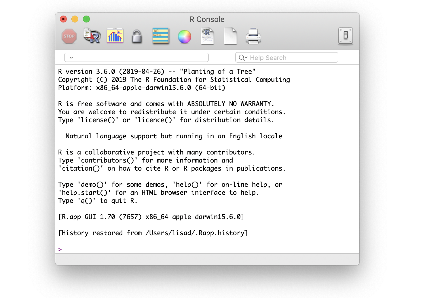
Figure 1.1: The R Console window.
You can close R and never open it again. We’ll be working entirely in RStudio in this class.
ALWAYS REMEMBER: Launch R though the RStudio IDE
Launch ![]() (RStudio.app), not
(RStudio.app), not ![]() (R.app).
(R.app).
1.3.2 RStudio
RStudio is an Integrated Development Environment (IDE). This is a program that serves as a text editor, file manager, and provides many functions to help you read and write R code.
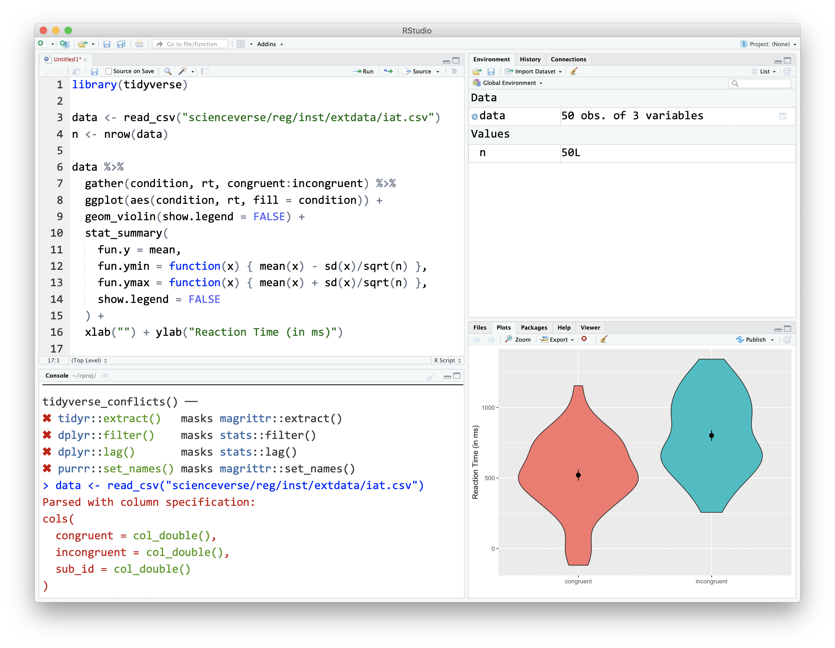
Figure 1.2: The RStudio IDE
RStudio is arranged with four window panes. By default, the upper left pane is the source pane, where you view and edit source code from files. The bottom left pane is usually the console pane, where you can type in commands and view output messages. The right panes have several different tabs that show you information about your code. You can change the location of panes and what tabs are shown under Preferences > Pane Layout.
1.3.3 Configure RStudio
In this class, you will be learning how to do reproducible research. This involves writing scripts that completely and transparently perform some analysis from start to finish in a way that yields the same result for different people using the same software on different computers. Transparency is a key value of science, as embodied in the “trust but verify” motto.

When you do things reproducibly, others can understand and check your work. This benefits science, but there is a selfish reason, too: the most important person who will benefit from a reproducible script is your future self. When you return to an analysis after two weeks of vacation, you will thank your earlier self for doing things in a transparent, reproducible way, as you can easily pick up right where you left off.
There are two tweaks that you should do to your RStudio installation to maximize reproducibility. Go to Global Options... under the Tools menu (⌘,), and uncheck the box that says Restore .RData into workspace at startup. If you keep things around in your workspace, things will get messy, and unexpected things will happen. You should always start with a clear workspace. This also means that you never want to save your workspace when you exit, so set this to Never. The only thing you want to save are your scripts.
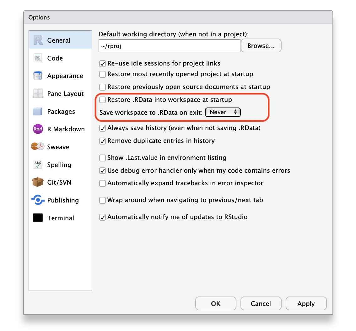
Figure 1.3: Alter these settings for increased reproducibility.
Your settings should have:
- Restore .RData into workspace at startup:
- Save workspace to .RData on exit:
1.4 Getting Started
1.4.1 Console commands
We are first going to learn about how to interact with the console. In general, you will be developing R script or R Markdown files, rather than working directly in the console window. However, you can consider the console a kind of “sandbox” where you can try out lines of code and adapt them until you get them to do what you want. Then you can copy them back into the script editor.
Mostly, however, you will be typing into the script editor window (either into an R script or an R Markdown file) and then sending the commands to the console by placing the cursor on the line and holding down the Ctrl key while you press Enter. The Ctrl+Enter key sequence sends the command in the script to the console.
One simple way to learn about the R console is to use it as a calculator. Enter the lines of code below and see if your results match. Be prepared to make lots of typos (at first).
1 + 1## [1] 2The R console remembers a history of the commands you typed in the past. Use the up and down arrow keys on your keyboard to scroll backwards and forwards through your history. It’s a lot faster than re-typing.
1 + 1 + 3## [1] 5You can break up mathematical expressions over multiple lines; R waits for a complete expression before processing it.
## here comes a long expression
## let's break it over multiple lines
1 + 2 + 3 + 4 + 5 + 6 +
    7 + 8 + 9 +
    10
## [1] 55Text inside quotes is called a string.
"Good afternoon"## [1] "Good afternoon"You can break up text over multiple lines; R waits for a close quote before processing it. If you want to include a double quote inside this quoted string, escape it with a backslash.
africa <- "I hear the drums echoing tonight
But she hears only whispers of some quiet conversation
She's coming in, 12:30 flight
The moonlit wings reflect the stars that guide me towards salvation
I stopped an old man along the way
Hoping to find some old forgotten words or ancient melodies
He turned to me as if to say, \"Hurry boy, it's waiting there for you\"

- Toto"

cat(africa) # cat() prints the string
## I hear the drums echoing tonight
## But she hears only whispers of some quiet conversation
## She's coming in, 12:30 flight
## The moonlit wings reflect the stars that guide me towards salvation
## I stopped an old man along the way
## Hoping to find some old forgotten words or ancient melodies
## He turned to me as if to say, "Hurry boy, it's waiting there for you"
##
## - Toto1.4.2 Objects
Often you want to store the result of some computation for later use. You can store it in an object (also sometimes called a variable). An object in R:
- contains only letters, numbers, full stops, and underscores
- starts with a letter or a full stop and a letter
- distinguishes uppercase and lowercase letters (
rickastleyis not the same asRickAstley)
The following are valid and different objects:
- songdata
- SongData
- song_data
- song.data
- .song.data
- never_gonna_give_you_up_never_gonna_let_you_down
The following are not valid objects:
- _song_data
- 1song
- .1song
- song data
- song-data
Use the assignment operator<-` to assign the value on the right to the object named on the left.
## use the assignment operator '<-'
## R stores the number in the object
x <- 5
Now that we have set x to a value, we can do something with it:
x * 2

## R evaluates the expression and stores the result in the object boring_calculation
boring_calculation <- 2 + 2
## [1] 10Note that it doesn’t print the result back at you when it’s stored. To view the result, just type the object name on a blank line.
boring_calculation## [1] 4Once an object is assigned a value, its value doesn’t change unless you reassign the object, even if the objects you used to calculate it change. Predict what the code below does and test yourself:
this_year <- 2019
my_birth_year <- 1976
my_age <- this_year - my_birth_year
this_year <- 2020
After all the code above is run:
this_year=my_birth_year=my_age=
1.4.3 The environment
Anytime you assign something to a new object, R creates a new entry in the global environment. Objects in the global environment exist until you end your session; then they disappear forever (unless you save them).
Look at the Environment tab in the upper right pane. It lists all of the objects you have created. Click the broom icon to clear all of the objects and start fresh. You can also use the following functions in the console to view all objects, remove one object, or remove all objects.
ls()            # print the objects in the global environment
rm("x")         # remove the object named x from the global environment
rm(list = ls()) # clear out the global environment
In the upper right corner of the Environment tab, change List to Grid. Now you can see the type, length, and size of your objects, and reorder the list by any of these attributes.
1.4.4 Whitespace
R mostly ignores whitespace: spaces, tabs, and line breaks. This means that you can use whitespace to help you organise your code.
# a and b are identical
a <- list(ctl = "Control Condition", exp1 = "Experimental Condition 1", exp2 = "Experimental Condition 2")

# but b is much easier to read
b <- list(ctl  = "Control Condition",
          exp1 = "Experimental Condition 1",
          exp2 = "Experimental Condition 2")
When you see > at the beginning of a line, that means R is waiting for you to start a new command. However, if you see a + instead of > at the start of the line, that means R is waiting for you to finish a command you started on a previous line. If you want to cancel whatever command you started, just press the Esc key in the console window and you’ll get back to the > command prompt.
# R waits until next line for evaluation
(3 + 2) *
     5
## [1] 25It is often useful to break up long functions onto several lines.
cat("3, 6, 9, the goose drank wine",
    "The monkey chewed tobacco on the streetcar line",
    "The line broke, the monkey got choked",
    "And they all went to heaven in a little rowboat",
    sep = "  \n")
## 3, 6, 9, the goose drank wine
## The monkey chewed tobacco on the streetcar line
## The line broke, the monkey got choked
## And they all went to heaven in a little rowboat1.4.5 Function syntax
A lot of what you do in R involves calling a function and storing the results. A function is a named section of code that can be reused.
For example, sd is a function that returns the standard deviation of the vector of numbers that you provide as the input argument. Functions are set up like this:
function_name(argument1, argument2 = "value").
The arguments in parentheses can be named (like, argument1 = 10) or you can skip the names if you put them in the exact same order that they’re defined in the function. You can check this by typing ?sd (or whatever function name you’re looking up) into the console and the Help pane will show you the default order under Usage. You can also skip arguments that have a default value specified.
Most functions return a value, but may also produce side effects like printing to the console.
To illustrate, the function rnorm() generates random numbers from the standard normal distribution. The help page for rnorm() (accessed by typing ?rnorm in the console) shows that it has the syntax
rnorm(n, mean = 0, sd = 1)
where n is the number of randomly generated numbers you want, mean is the mean of the distribution, and sd is the standard deviation. The default mean is 0, and the default standard deviation is 1. There is no default for n, which means you’ll get an error if you don’t specify it:
rnorm()## Error in rnorm(): argument "n" is missing, with no defaultIf you want 10 random numbers from a normal distribution with mean of 0 and standard deviation, you can just use the defaults.
rnorm(10)## [1] -0.04234663 -2.00393149 0.83611187 -1.46404127 1.31714428 0.42608581
## [7] -0.46673798 -0.01670509 1.64072295 0.85876439If you want 10 numbers from a normal distribution with a mean of 100:
rnorm(10, 100)## [1] 101.34917 99.86059 100.36287 99.65575 100.66818 100.04771 99.76782
## [8] 102.57691 100.05575 99.42490This would be an equivalent but less efficient way of calling the function:
rnorm(n = 10, mean = 100)## [1] 100.52773 99.40241 100.39641 101.01629 99.41961 100.52202 98.09828
## [8] 99.52169 100.25677 99.92092We don’t need to name the arguments because R will recognize that we intended to fill in the first and second arguments by their position in the function call. However, if we want to change the default for an argument coming later in the list, then we need to name it. For instance, if we wanted to keep the default mean = 0 but change the standard deviation to 100 we would do it this way:
rnorm(10, sd = 100)## [1] -68.254349 -17.636619 140.047575 7.570674 -68.309751 -2.378786
## [7] 117.356343 -104.772092 -40.163750 54.358941Some functions give a list of options after an argument; this means the default value is the first option. The usage entry for the power.t.test() function looks like this:
power.t.test(n = NULL, delta = NULL, sd = 1, sig.level = 0.05,
             power = NULL,
             type = c("two.sample", "one.sample", "paired"),
             alternative = c("two.sided", "one.sided"),
strict = FALSE, tol = .Machine$double.eps^0.25)- What is the default value for
sd? - What is the default value for
type? - Which is equivalent to
power.t.test(100, 0.5)?
1.4.6 Getting help
Start up help in a browser using the function help.start().
If a function is in base R or a loaded package, you can use the help("function_name") function or the ?function_name shortcut to access the help file. If the package isn’t loaded, specify the package name as the second argument to the help function.
# these methods are all equivalent ways of getting help
help("rnorm")
?rnorm
help("rnorm", package="stats")
When the package isn’t loaded or you aren’t sure what package the function is in, use the shortcut ??function_name.
- What is the first argument to the
meanfunction? - What package is
read_excelin?
1.5 Add-on packages
One of the great things about R is that it is user extensible: anyone can create a new add-on software package that extends its functionality. There are currently thousands of add-on packages that R users have created to solve many different kinds of problems, or just simply to have fun. There are packages for data visualisation, machine learning, neuroimaging, eyetracking, web scraping, and playing games such as Sudoku.
Add-on packages are not distributed with base R, but have to be downloaded and installed from an archive, in the same way that you would, for instance, download and install a fitness app on your smartphone.
The main repository where packages reside is called CRAN, the Comprehensive R Archive Network. A package has to pass strict tests devised by the R core team to be allowed to be part of the CRAN archive. You can install from the CRAN archive through R using the install.packages() function.
There is an important distinction between installing a package and loading a package.
1.5.1 Installing a package

This is done using install.packages(). This is like installing an app on your phone: you only have to do it once and the app will remain installed until you remove it. For instance, if you want to use PokemonGo on your phone, you install it once from the App Store or Play Store, and you don’t have to re-install it each time you want to use it. Once you launch the app, it will run in the background until you close it or restart your phone. Likewise, when you install a package, the package will be available (but not loaded) every time you open up R.
You may only be able to permanently install packages if you are using R on your own system; you may not be able to do this on public workstations if you lack the appropriate privileges.
Install the ggExtra package on your system. This package lets you create plots with marginal histograms.
install.packages("ggExtra")If you don’t already have packages like ggplot2 and shiny installed, it will also install these dependencies for you. If you don’t get an error message at the end, the installation was successful.
1.5.2 Loading a package
This is done using library(packagename). This is like launching an app on your phone: the functionality is only there where the app is launched and remains there until you close the app or restart. Likewise, when you run library(packagename) within a session, the functionality of the package referred to by packagename will be made available for your R session. The next time you start R, you will need to run the library() function again if you want to access its functionality.
You can load the functions in ggExtra for your current R session as follows:
library(ggExtra)You might get some red text when you load a package, this is normal. It is usually warning you that this package has functions that have the same name as other packages you’ve already loaded.
You can use the convention package::function() to indicate in which add-on package a function resides. For instance, if you see readr::read_csv(), that refers to the function read_csv() in the readr add-on package.
Now you can run the function ggExtra::runExample(), which runs an interactive example of marginal plots using shiny.
ggExtra::runExample()1.5.3 Install from GitHub
Many R packages are not yet on CRAN because they are still in development. Increasingly, datasets and code for papers are available as packages you can download from github. You’ll need to install the devtools package to be able to install packages from github. Check if you have a package installed by trying to load it (e.g., if you don’t have devtools installed, library("devtools") will display an error message) or by searching for it in the packages tab in the lower right pane. All listed packages are installed; all checked packages are currently loaded.
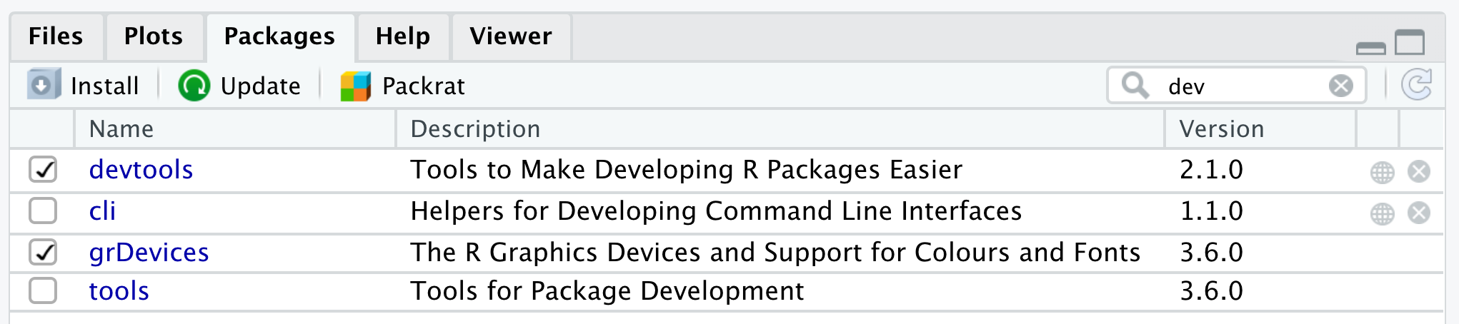
Figure 1.4: Check installed and loaded packages in the packages tab in the lower right pane.
# install devtools if you get
# Error in loadNamespace(name) : there is no package called ‘devtools’
# install.packages("devtools")
devtools::install_github("psyteachr/msc-data-skills")
After you install the dataskills package, load it using the library() function. You can then try out some of the functions below.
book()opens a local copy of this book in your web browser.app("plotdemo")opens a shiny app that lets you see how simulated data would look in different plot stylesexercise(1)creates and opens a file containing the exercises for this chapter?disgustshows you the documentation for the built-in datasetdisgust, which we will be using in future lessons
library(dataskills)
book()
app("plotdemo")
exercise(1)
?disgust
How many different ways can you find to discover what functions are available in the dataskills package?
1.6 Organising a project
Projects in RStudio are a way to group all of the files you need for one project. Most projects include scripts, data files, and output files like the PDF version of the script or images.
Make a new directory where you will keep all of your materials for this class. If you’re using a lab computer, make sure you make this directory in your network drive so you can access it from other computers.
Choose New Project… under the File menu to create a new project called 01-intro in this directory.
1.6.1 Structure
Here is what an R script looks like. Don’t worry about the details for now.
# load add-on packages
library(tidyverse)

# set object ----
n <- 100

# simulate data ----
data <- data.frame(
  id = 1:n,
  dv = c(rnorm(n/2, 0), rnorm(n/2, 1)),
  condition = rep(c("A", "B"), each = n/2)
)

# plot data ----
ggplot(data, aes(condition, dv)) +
  geom_violin(trim = FALSE) +
  geom_boxplot(width = 0.25,
               aes(fill = condition),
               show.legend = FALSE)

# save plot ----
ggsave("sim_data.png", width = 8, height = 6)
It’s best if you follow the following structure when developing your own scripts:
- load in any add-on packages you need to use
- define any custom functions
- load or simulate the data you will be working with
- work with the data
- save anything you need to save
Often when you are working on a script, you will realize that you need to load another add-on package. Don’t bury the call to library(package_I_need) way down in the script. Put it in the top, so the user has an overview of what packages are needed.
You can add comments to an R script by with the hash symbol (#). The R interpreter will ignore characters from the hash to the end of the line.
## comments: any text from '#' on is ignored until end of line
22 / 7  # approximation to pi
## [1] 3.142857If you add 4 or more dashes to the end of a comment, it acts like a header and creates an outline that you can see in the document outline (⇧⌘O).
1.6.2 Reproducible reports with R Markdown
We will make reproducible reports following the principles of literate programming. The basic idea is to have the text of the report together in a single document along with the code needed to perform all analyses and generate the tables. The report is then “compiled” from the original format into some other, more portable format, such as HTML or PDF. This is different from traditional cutting and pasting approaches where, for instance, you create a graph in Microsoft Excel or a statistics program like SPSS and then paste it into Microsoft Word.
We will use R Markdown to create reproducible reports, which enables mixing of text and code. A reproducible script will contain sections of code in code blocks. A code block starts and ends with backtick symbols in a row, with some infomation about the code between curly brackets, such as {r chunk-name, echo=FALSE} (this runs the code, but does not show the text of the code block in the compiled document). The text outside of code blocks is written in markdown, which is a way to specify formatting, such as headers, paragraphs, lists, bolding, and links.
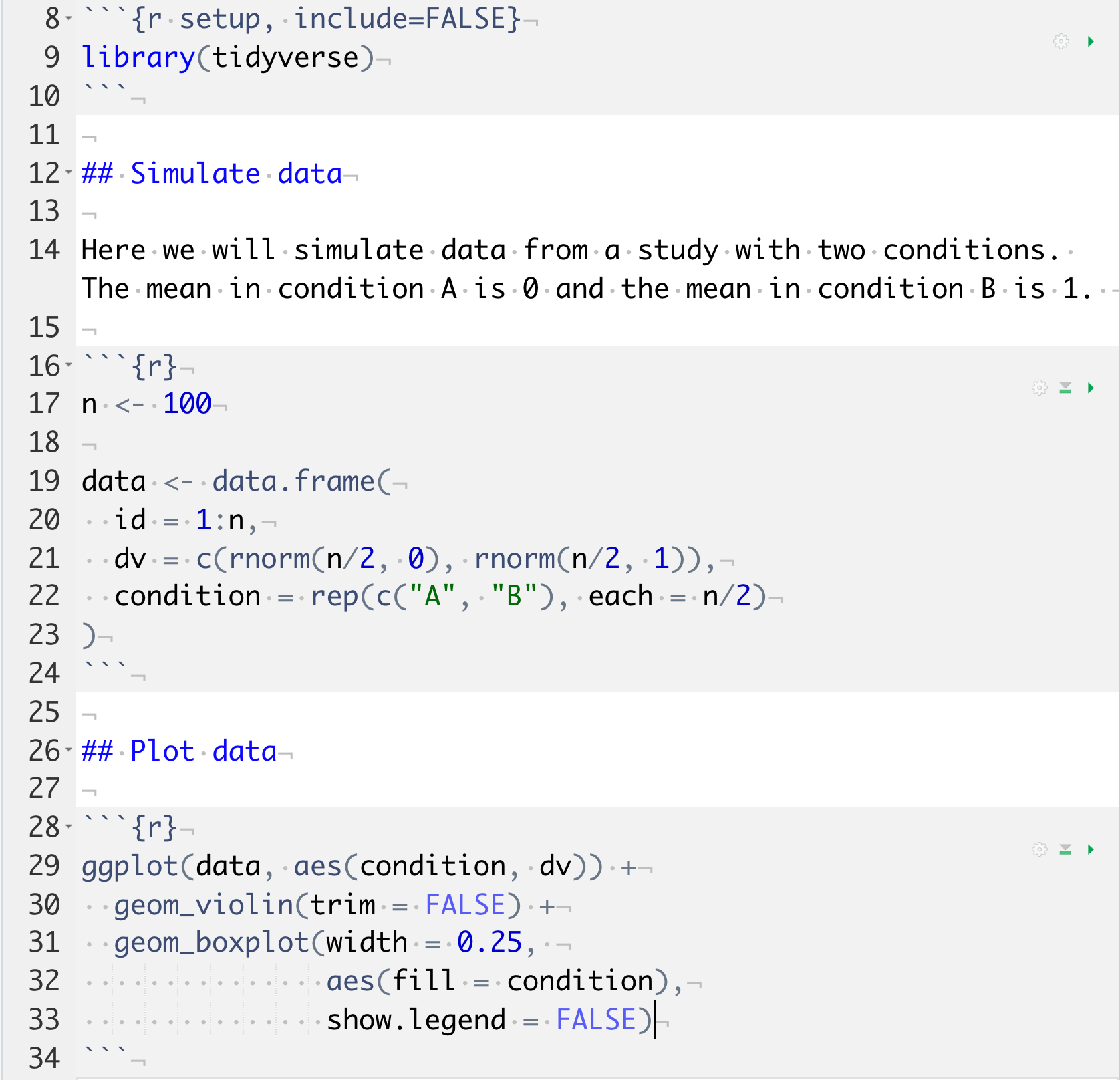
Figure 1.5: A reproducible script.
If you open up a new R Markdown file from a template, you will see an example document with several code blocks in it. To create an HTML or PDF report from an R Markdown (Rmd) document, you compile it. Compiling a document is called knitting in RStudio. There is a button that looks like a ball of yarn with needles through it that you click on to compile your file into a report.
Create a new R Markdown file from the File > New File > R Markdown… menu. Change the title and author, then click the knit button to create an html file.
1.6.3 Working Directory
Where should you put all of your files? When developing an analysis, you usually want to have all of your scripts and data files in one subtree of your computer’s directory structure. Usually there is a single working directory where your data and scripts are stored.
Your script should only reference files in three locations, using the appropriate format.
| Where | Example |
|---|---|
| on the web | “https://psyteachr.github.io/msc-data-skills/data/disgust_scores.csv” |
| in the working directory | “disgust_scores.csv” |
| in a subdirectory | “data/disgust_scores.csv” |
Never set or change your working directory in a script.
If you are working with an R Markdown file, it will automatically use the same directory the .Rmd file is in as the working directory.
If you are working with R scripts, store your main script file in the top-level directory and manually set your working directory to that location. You will have to reset the working directory each time you open RStudio, unless you create a project and access the script from the project.
For instance, if you are on a Windows machine your data and scripts are in the directory C:\Carla's_files\thesis2\my_thesis\new_analysis, you will set your working directory in one of two ways: (1) by going to the Session pull down menu in RStudio and choosing Set Working Directory, or (2) by typing setwd("C:\Carla's_files\thesis2\my_thesis\new_analysis") in the console window.
It’s tempting to make your life simple by putting the setwd() command in your script. Don’t do this! Others will not have the same directory tree as you (and when your laptop dies and you get a new one, neither will you).
When manually setting the working directory, always do so by using the Session > Set Working Directory pull-down option or by typing setwd() in the console.
If your script needs a file in a subdirectory of new_analysis, say, data/questionnaire.csv, load it in using a relative path so that it is accessible if you move the folder new_analysis to another location or computer:
dat <- read_csv("data/questionnaire.csv") # correctDo not load it in using an absolute path:
dat <- read_csv("C:/Carla's_files/thesis22/my_thesis/new_analysis/data/questionnaire.csv") # wrongAlso note the convention of using forward slashes, unlike the Windows-specific convention of using backward slashes. This is to make references to files platform independent.
1.7 Glossary
Each chapter ends with a glossary table defining the jargon introduced in this chapter. The links below take you to the glossary book, which you can also download for offline use with devtools::install_github("psyteachr/glossary") and access the glossary offline with glossary::book().
| term | definition |
|---|---|
| absolute path | A file path that starts with / and is not appended to the working directory |
| argument | A variable that provides input to a function. |
| assignment operator | The symbol <-, which functions like = and assigns the value on the right to the object on the left |
| base r | The set of R functions that come with a basic installation of R, before you add external packages |
| console | The pane in RStudio where you can type in commands and view output messages. |
| cran | The Comprehensive R Archive Network: a network of ftp and web servers around the world that store identical, up-to-date, versions of code and documentation for R. |
| escape | Include special characters like " inside of a string by prefacing them with a backslash. |
| function | A named section of code that can be reused. |
| global environment | The interactive workspace where your script runs |
| ide | Integrated Development Environment: a program that serves as a text editor, file manager, and provides functions to help you read and write code. RStudio is an IDE for R. |
| knit | To create an HTML, PDF, or Word document from an R Markdown (Rmd) document |
| markdown | A way to specify formatting, such as headers, paragraphs, lists, bolding, and links. |
| normal distribution | A symmetric distribution of data where values near the centre are most probable. |
| object | A word that identifies and stores the value of some data for later use. |
| package | A group of R functions. |
| panes | RStudio is arranged with four window “panes.” |
| project | A way to organise related files in RStudio |
| r markdown | The R-specific version of markdown: a way to specify formatting, such as headers, paragraphs, lists, bolding, and links, as well as code blocks and inline code. |
| relative path | The location of a file in relation to the working directory. |
| reproducible research | Research that documents all of the steps between raw data and results in a way that can be verified. |
| script | A plain-text file that contains commands in a coding language, such as R. |
| scripts | NA |
| standard deviation | A descriptive statistic that measures how spread out data are relative to the mean. |
| string | A piece of text inside of quotes. |
| variable | A word that identifies and stores the value of some data for later use. |
| vector | A type of data structure that is basically a list of things like T/F values, numbers, or strings. |
| whitespace | Spaces, tabs and line breaks |
| working directory | The filepath where R is currently reading and writing files. |
1.8 Exercises
Download the first set of exercises and put it in the project directory you created earlier for today’s exercises. See the answers only after you’ve attempted all the questions.
# run this to access the exercise
dataskills::exercise(1)

# run this to access the answers
dataskills::exercise(1, answers = TRUE)