C Styling Plots
C.1 Aesthetics
C.1.1 Colour/Fill
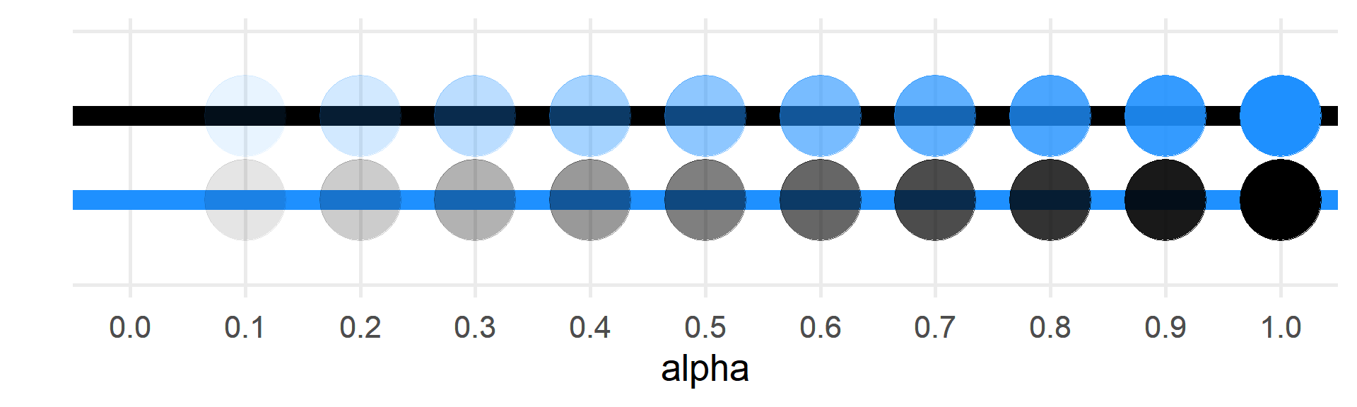
The colour argument changes the point and line colour, while the fill argument changes the interior colour of shapes. Type colours() into the console to see a list of all the named colours in R. Alternatively, you can use hexadecimal colours like "#FF8000" or the rgb() function to set red, green, and blue values on a scale from 0 to 1.
Hover over a colour to see its R name.
- black
- gray1
- gray2
- gray3
- gray4
- gray5
- gray6
- gray7
- gray8
- gray9
- gray10
- gray11
- gray12
- gray13
- gray14
- gray15
- gray16
- gray17
- gray18
- gray19
- gray20
- gray21
- gray22
- gray23
- gray24
- gray25
- gray26
- gray27
- gray28
- gray29
- gray30
- gray31
- gray32
- gray33
- gray34
- gray35
- gray36
- gray37
- gray38
- gray39
- gray40
- dimgray
- gray42
- gray43
- gray44
- gray45
- gray46
- gray47
- gray48
- gray49
- gray50
- gray51
- gray52
- gray53
- gray54
- gray55
- gray56
- gray57
- gray58
- gray59
- gray60
- gray61
- gray62
- gray63
- gray64
- gray65
- darkgray
- gray66
- gray67
- gray68
- gray69
- gray70
- gray71
- gray72
- gray73
- gray74
- gray
- gray75
- gray76
- gray77
- gray78
- gray79
- gray80
- gray81
- gray82
- gray83
- lightgray
- gray84
- gray85
- gainsboro
- gray86
- gray87
- gray88
- gray89
- gray90
- gray91
- gray92
- gray93
- gray94
- gray95
- gray96
- gray97
- gray98
- gray99
- white
- snow4
- snow3
- snow2
- snow
- rosybrown4
- rosybrown
- rosybrown3
- rosybrown2
- rosybrown1
- lightcoral
- indianred
- indianred4
- indianred2
- indianred1
- indianred3
- brown4
- brown
- brown3
- brown2
- brown1
- firebrick4
- firebrick
- firebrick3
- firebrick1
- firebrick2
- darkred
- red3
- red2
- red
- mistyrose3
- mistyrose4
- mistyrose2
- mistyrose
- salmon
- tomato3
- coral4
- coral3
- coral2
- coral1
- tomato2
- tomato
- tomato4
- darksalmon
- salmon4
- salmon3
- salmon2
- salmon1
- coral
- orangered4
- orangered3
- orangered2
- lightsalmon3
- lightsalmon2
- lightsalmon
- lightsalmon4
- sienna
- sienna3
- sienna2
- sienna1
- sienna4
- orangered
- seashell4
- seashell3
- seashell2
- seashell
- chocolate4
- chocolate3
- chocolate
- chocolate2
- chocolate1
- linen
- peachpuff4
- peachpuff3
- peachpuff2
- peachpuff
- sandybrown
- tan4
- peru
- tan2
- tan1
- darkorange4
- darkorange3
- darkorange2
- darkorange1
- antiquewhite3
- antiquewhite2
- antiquewhite1
- bisque4
- bisque3
- bisque2
- bisque
- burlywood4
- burlywood3
- burlywood
- burlywood2
- burlywood1
- darkorange
- antiquewhite4
- antiquewhite
- papayawhip
- blanchedalmond
- navajowhite4
- navajowhite3
- navajowhite2
- navajowhite
- tan
- floralwhite
- oldlace
- wheat4
- wheat3
- wheat2
- wheat
- wheat1
- moccasin
- orange4
- orange3
- orange2
- orange
- goldenrod
- goldenrod1
- goldenrod4
- goldenrod3
- goldenrod2
- darkgoldenrod4
- darkgoldenrod
- darkgoldenrod3
- darkgoldenrod2
- darkgoldenrod1
- cornsilk
- cornsilk4
- cornsilk3
- cornsilk2
- lightgoldenrod4
- lightgoldenrod3
- lightgoldenrod
- lightgoldenrod2
- lightgoldenrod1
- gold4
- gold3
- gold2
- gold
- lemonchiffon4
- lemonchiffon3
- lemonchiffon2
- lemonchiffon
- palegoldenrod
- khaki
- darkkhaki
- khaki4
- khaki3
- khaki2
- khaki1
- ivory4
- ivory3
- ivory2
- ivory
- beige
- lightyellow4
- lightyellow3
- lightyellow2
- lightyellow
- lightgoldenrodyellow
- yellow4
- yellow3
- yellow2
- yellow
- olivedrab
- olivedrab4
- olivedrab3
- olivedrab2
- olivedrab1
- darkolivegreen
- darkolivegreen4
- darkolivegreen3
- darkolivegreen2
- darkolivegreen1
- greenyellow
- chartreuse4
- chartreuse3
- chartreuse2
- lawngreen
- chartreuse
- honeydew4
- honeydew3
- honeydew2
- honeydew
- darkseagreen4
- darkseagreen
- darkseagreen3
- darkseagreen2
- darkseagreen1
- lightgreen
- palegreen
- palegreen4
- palegreen3
- palegreen1
- forestgreen
- limegreen
- darkgreen
- green4
- green3
- green2
- green
- mediumseagreen
- seagreen
- seagreen3
- seagreen2
- seagreen1
- mintcream
- springgreen4
- springgreen3
- springgreen2
- springgreen
- aquamarine3
- aquamarine2
- aquamarine
- mediumspringgreen
- aquamarine4
- turquoise
- mediumturquoise
- lightseagreen
- azure4
- azure3
- azure2
- azure
- lightcyan4
- lightcyan3
- lightcyan2
- lightcyan
- paleturquoise
- paleturquoise4
- paleturquoise3
- paleturquoise2
- paleturquoise1
- darkslategray
- darkslategray4
- darkslategray3
- darkslategray2
- darkslategray1
- cyan4
- cyan3
- darkturquoise
- cyan2
- cyan
- cadetblue4
- cadetblue
- turquoise4
- turquoise3
- turquoise2
- turquoise1
- powderblue
- cadetblue3
- cadetblue2
- cadetblue1
- lightblue4
- lightblue3
- lightblue
- lightblue2
- lightblue1
- deepskyblue4
- deepskyblue3
- deepskyblue2
- deepskyblue
- skyblue
- lightskyblue4
- lightskyblue3
- lightskyblue2
- lightskyblue1
- lightskyblue
- skyblue4
- skyblue3
- skyblue2
- skyblue1
- aliceblue
- slategray
- lightslategray
- slategray3
- slategray2
- slategray1
- steelblue4
- steelblue
- steelblue3
- steelblue2
- steelblue1
- dodgerblue4
- dodgerblue3
- dodgerblue2
- dodgerblue
- lightsteelblue4
- lightsteelblue3
- lightsteelblue
- lightsteelblue2
- lightsteelblue1
- slategray4
- cornflowerblue
- royalblue
- royalblue4
- royalblue3
- royalblue2
- royalblue1
- ghostwhite
- lavender
- midnightblue
- navy
- blue4
- blue3
- blue2
- blue
- darkslateblue
- slateblue
- mediumslateblue
- lightslateblue
- slateblue1
- slateblue4
- slateblue3
- slateblue2
- mediumpurple4
- mediumpurple3
- mediumpurple
- mediumpurple2
- mediumpurple1
- purple4
- purple3
- blueviolet
- purple1
- purple2
- purple
- darkorchid
- darkorchid4
- darkorchid3
- darkorchid2
- darkorchid1
- darkviolet
- mediumorchid4
- mediumorchid3
- mediumorchid
- mediumorchid2
- mediumorchid1
- thistle4
- thistle3
- thistle
- thistle2
- thistle1
- plum4
- plum3
- plum2
- plum1
- plum
- violet
- darkmagenta
- magenta3
- magenta2
- magenta
- orchid4
- orchid3
- orchid
- orchid2
- orchid1
- maroon4
- violetred
- maroon3
- maroon2
- maroon1
- mediumvioletred
- deeppink3
- deeppink2
- deeppink
- deeppink4
- hotpink2
- hotpink1
- hotpink4
- hotpink
- violetred4
- violetred3
- violetred2
- violetred1
- hotpink3
- lavenderblush4
- lavenderblush3
- lavenderblush2
- lavenderblush
- maroon
- palevioletred4
- palevioletred3
- palevioletred
- palevioletred2
- palevioletred1
- pink4
- pink3
- pink2
- pink1
- pink
- lightpink
- lightpink4
- lightpink3
- lightpink2
- lightpink1
C.2 Palettes
Discrete palettes change depending on the number of categories.
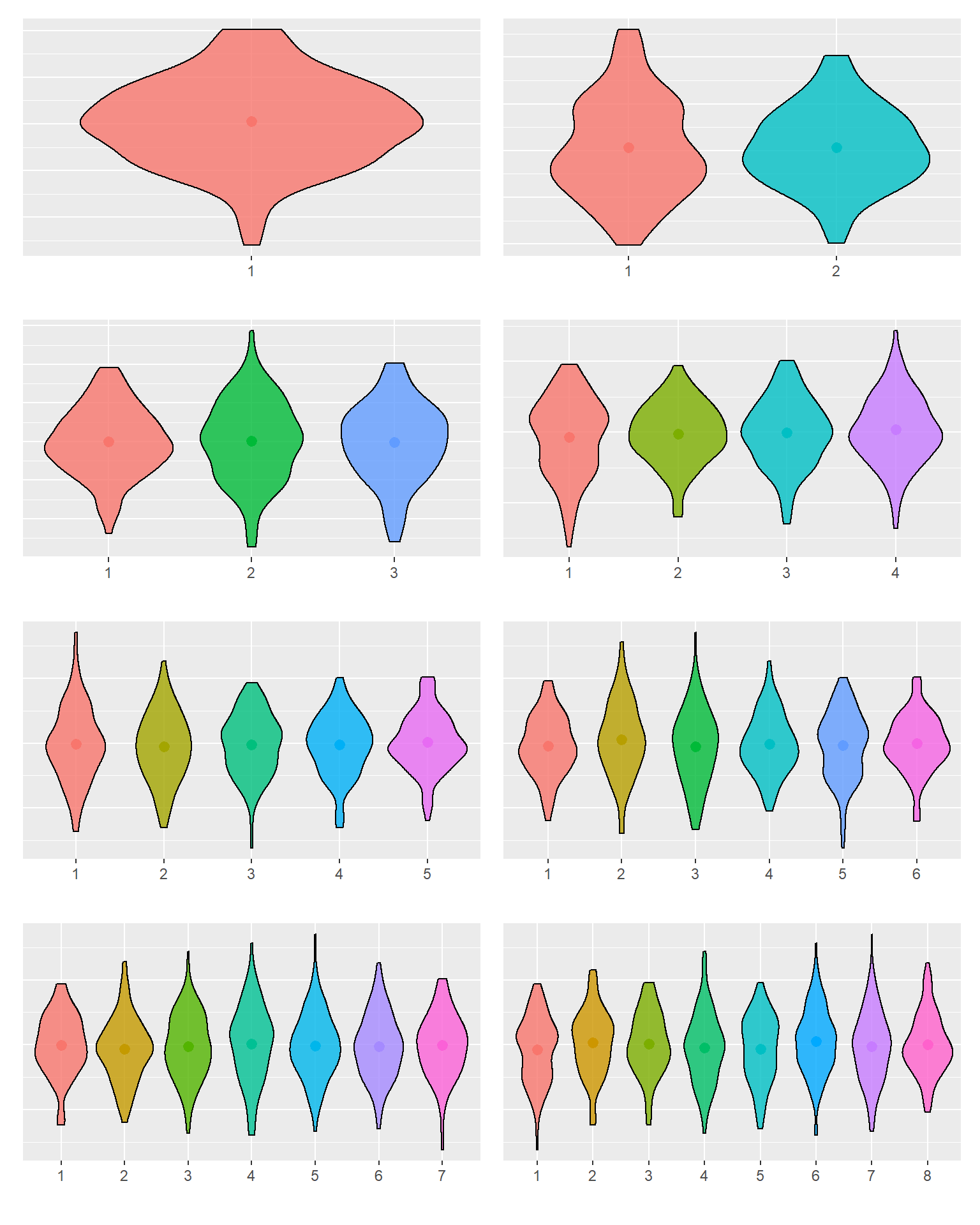
Figure C.4: Default discrete palette with different numbers of levels.
C.2.1 Viridis Palettes
Viridis palettes are very good for colourblind-safe and greyscale-safe plots. The work with any number of categories, but are best for larger numbers of categories or continuous colours.
C.2.1.1 Discrete Viridis Palettes
Set discrete viridis colours with scale_colour_viridis_d() or scale_fill_viridis_d() and set the option argument to one of the options below. Set direction = -1 to reverse the order of colours.
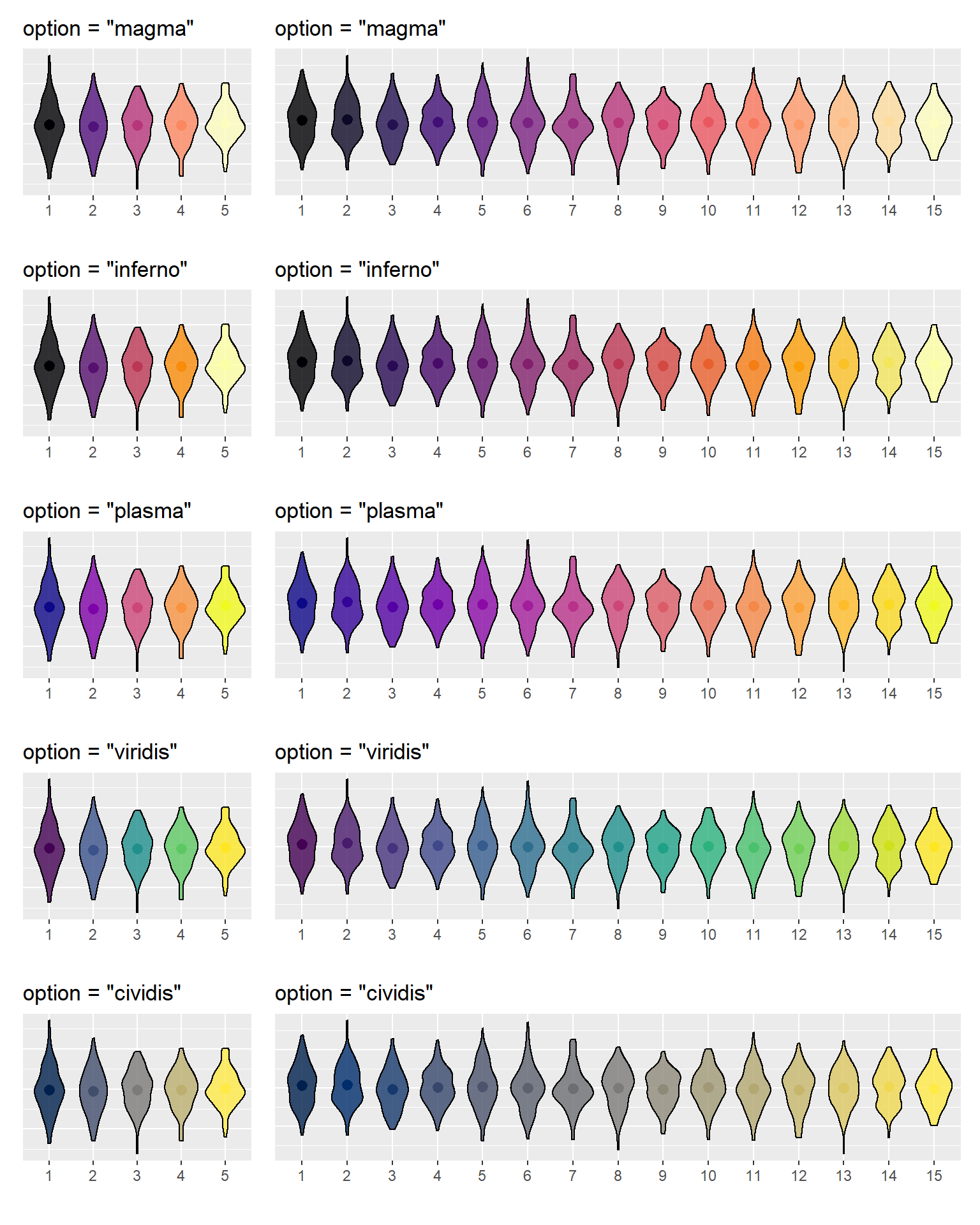
Figure C.5: Discrete viridis palettes.
If the end colour is too light for your plot or the start colour too dark, you can set the begin and end arguments to values between 0 and 1, such as scale_colour_viridis_c(begin = 0.1, end = 0.9).
C.2.1.2 Continuous Viridis Palettes
Set continuous viridis colours with scale_colour_viridis_c() or scale_fill_viridis_c() and set the option argument to one of the options below. Set direction = -1 to reverse the order of colours.
Figure 3.7: Continuous viridis palettes.
C.2.2 Brewer Palettes
Brewer palettes give you a lot of control over plot colour and fill. You set them with scale_color_brewer() or scale_fill_brewer() and set the palette argument to one of the palettes below. Set direction = -1 to reverse the order of colours.
C.2.2.1 Qualitative Brewer Palettes
These palettes are good for categorical data with up to 8 categories (some palettes can handle up to 12). The "Paired" palette is useful if your categories are arranged in pairs.
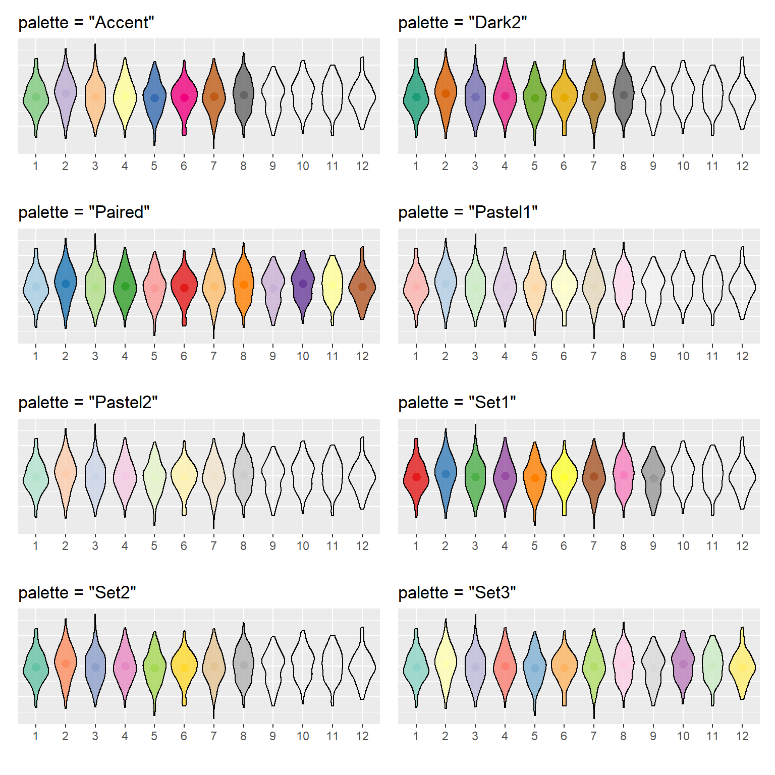
Figure C.6: Qualitative brewer palettes.
C.2.2.2 Sequential Brewer Palettes
These palettes are good for up to 9 ordinal categories with a lot of categories.
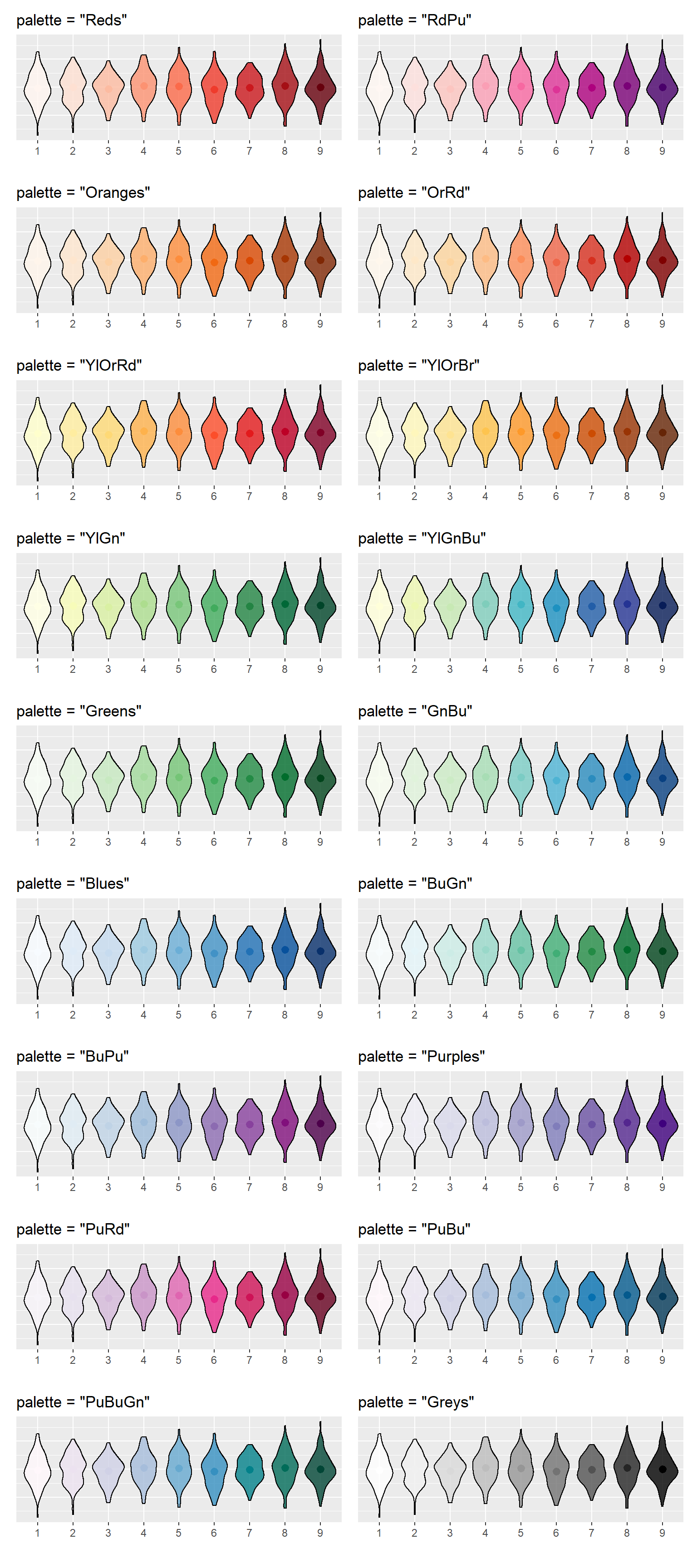
Figure C.7: Sequential brewer palettes.
C.2.2.3 Diverging Brewer Palettes
These palettes are good for ordinal categories with up to 11 levels where the centre level is a neutral or baseline category and the levels above and below it differ in an important way, such as agree versus disagree options.
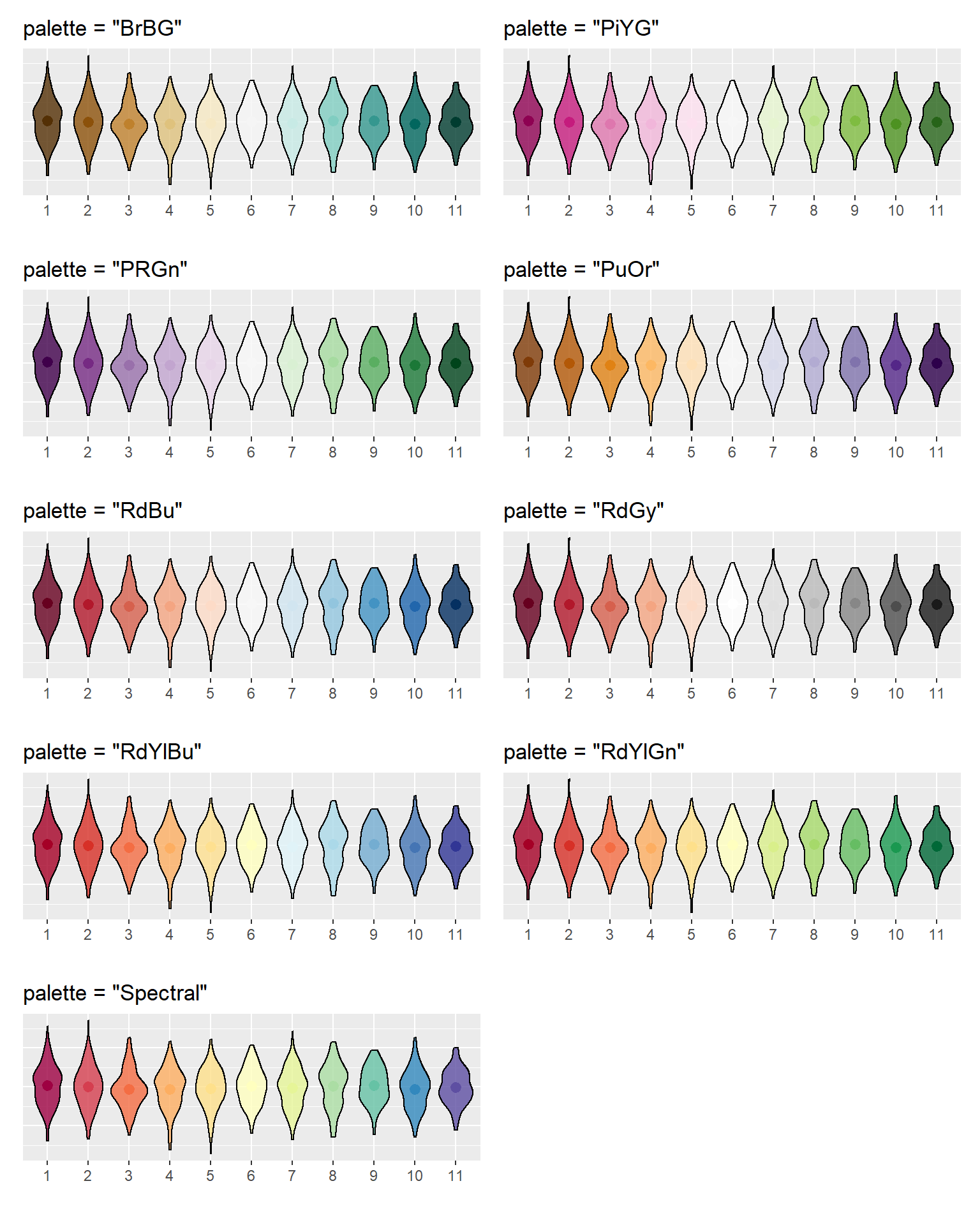
Figure C.8: Diverging brewer palettes.
C.3 Themes
ggplot2 has 8 built-in themes that you can add to a plot like plot + theme_bw() or set as the default theme at the top of your script like theme_set(theme_bw()).
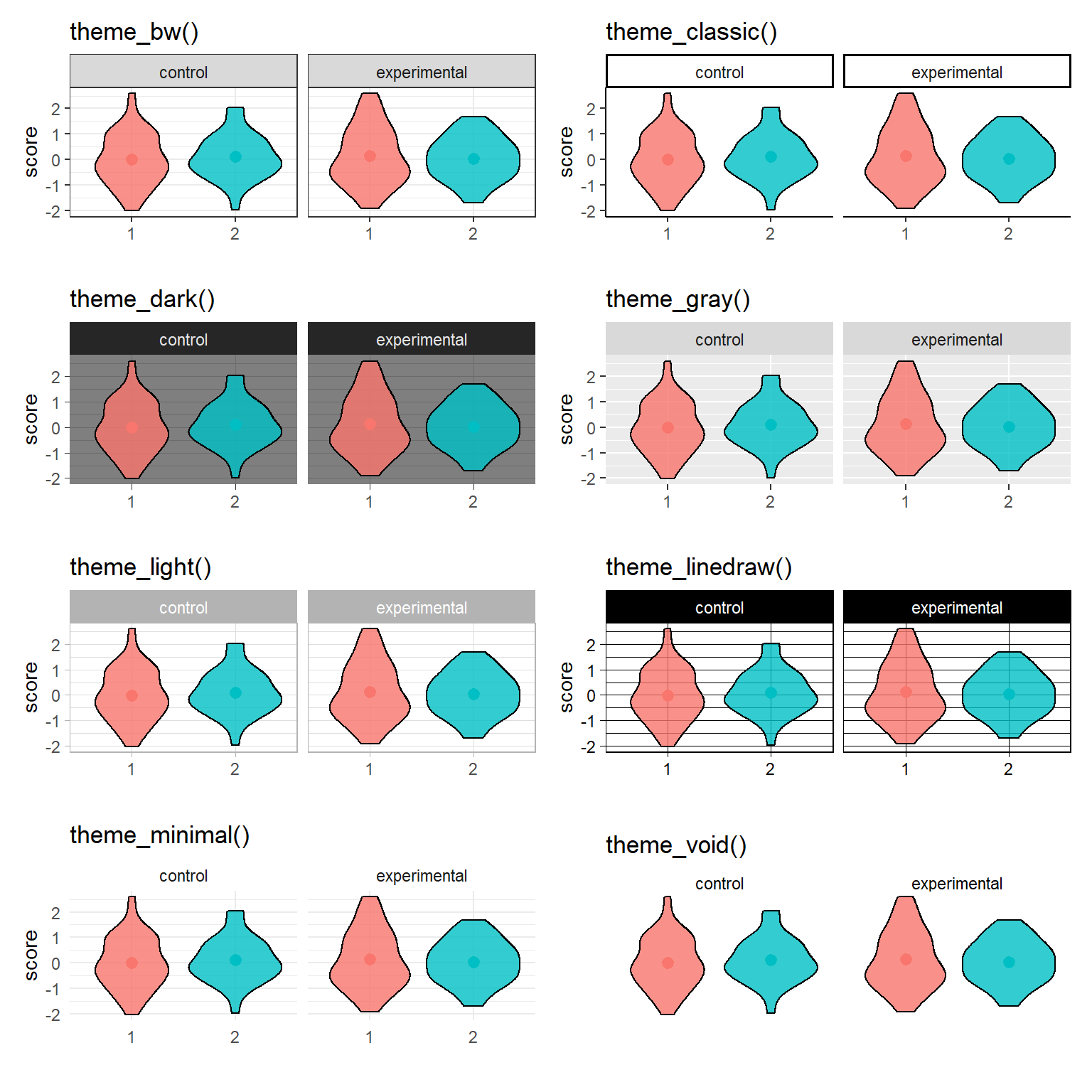
Figure C.9: {ggplot2} themes.
C.3.1 ggthemes
You can get more themes from add-on packages, like ggthemes. Most of the themes also have custom scale_ functions like scale_colour_economist(). Their website has extensive examples and instructions for alternate or dark versions of these themes.
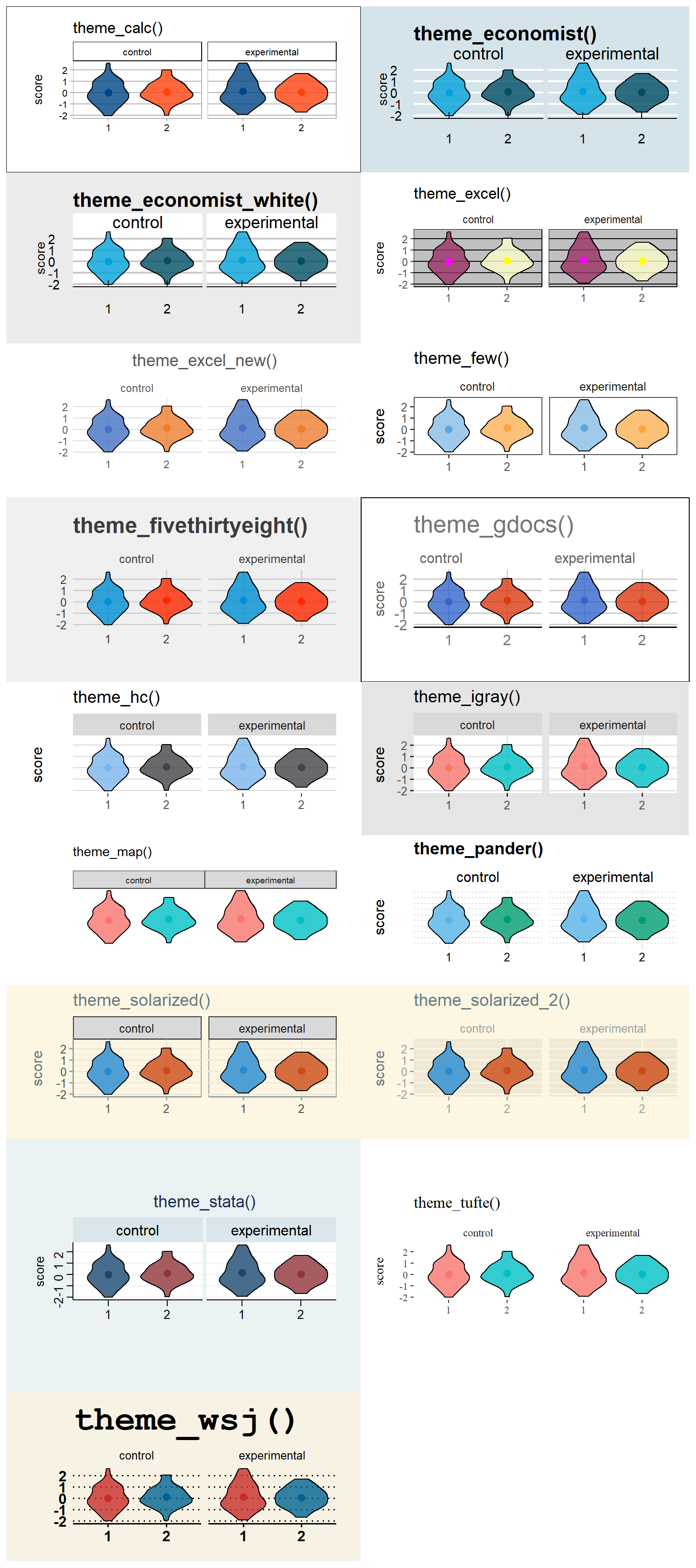
Figure C.10: {ggthemes} themes.
C.3.2 Fonts
You can customise the fonts used in themes. All computers should be able to recognise the families "sans", "serif", and "mono", and some computers will be able to access other installed fonts by name.
sans <- g + theme_bw(base_family = "sans") +
  ggtitle("Sans")
serif <- g + theme_bw(base_family = "serif") +
  ggtitle("Serif")
mono <- g + theme_bw(base_family = "mono") +
  ggtitle("Mono")
font <- g + theme_bw(base_family = "Comic Sans MS") +
  ggtitle("Comic Sans MS")

sans + serif + mono + font + plot_layout(nrow = 1)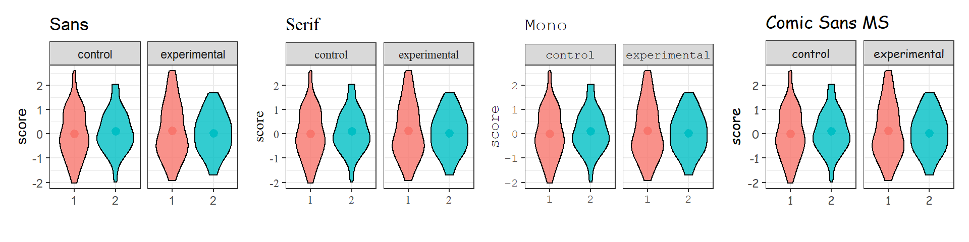
Figure C.11: Different fonts.
If you are working on a Windows machine and get the error "font family not found in Windows font database", you may need to explicitly map the fonts. In your setup code chunk, add the following code, which should fix the error. You may need to do this for any fonts that you specify.
The showtext package is a flexible way to add fonts.
If you have a .ttf file from a font site, like Font Squirrel, you can load the file directly using font_add(). Set regular as the path to the file for the regular version of the font, and optionally add other versions. Set the family to the name you want to use for the font. You will need to include any local font files if you are sharing your script with others.
library(showtext)

# font from https://www.fontsquirrel.com/fonts/SF-Cartoonist-Hand

font_add(
  regular = "fonts/cartoonist/SF_Cartoonist_Hand.ttf",
  bold = "fonts/cartoonist/SF_Cartoonist_Hand_Bold.ttf",
  italic = "fonts/cartoonist/SF_Cartoonist_Hand_Italic.ttf",
  bolditalic = "fonts/cartoonist/SF_Cartoonist_Hand_Bold_Italic.ttf",
  family = "cartoonist"
)
To download fonts directly from Google fonts, use the function font_add_google(), set the name to the exact name from the site, and the family to the name you want to use for the font.
# download fonts from Google
font_add_google(name = "Courgette", family = "courgette")
font_add_google(name = "Poiret One", family = "poiret")
After you've added fonts from local files or Google, you need to make them available to R using showtext_auto(). You will have to do these steps in each script where you want to use the custom fonts.
showtext_auto() # load the fontsTo change the fonts used overall in a plot, use the theme() function and set text to element_text(family = "new_font_family").
a <- g + theme(text = element_text(family = "courgette")) +
  ggtitle("Courgette")
b <- g + theme(text = element_text(family = "cartoonist")) +
  ggtitle("Cartoonist Hand")
c <- g + theme(text = element_text(family = "poiret")) +
  ggtitle("Poiret One")

a + b + c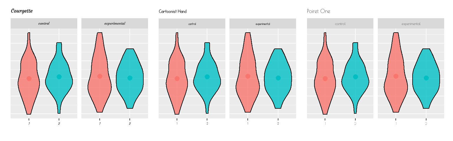
Figure C.12: Custom Fonts.
To set the fonts for individual elements in the plot, you need to find the specific argument for that element. You can use the argument face to choose "bold", "italic", or "bolditalic" versions, if they are available.
g + ggtitle("Cartoonist Hand") +
  theme(
    title = element_text(family = "cartoonist", face = "bold"),
    strip.text = element_text(family = "cartoonist", face = "italic"),
    axis.text = element_text(family = "sans")
  )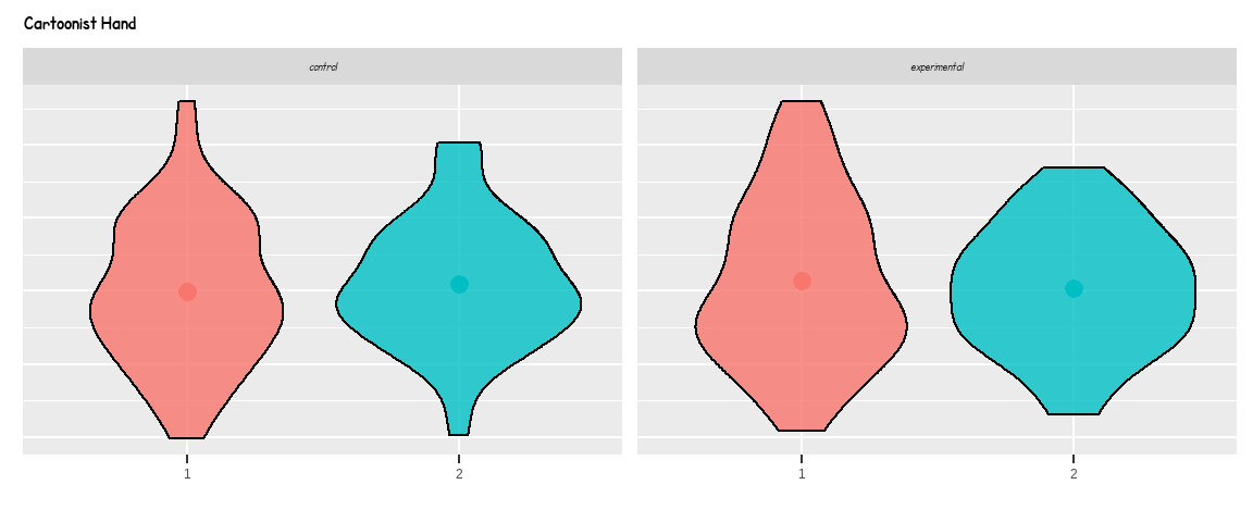
Figure C.13: Multiple custom fonts on the same plot.
C.3.3 Setting A Lab Theme using theme()
The theme() function, as we mentioned, does a lot more than just change the position of a legend and can be used to really control a variety of elements and to eventually create your own "theme" for your figures - say you want to have a consistent look to your figures across your publications or across your lab posters.
First, we'll create a basic plot to demonstrate the changes.
g <- ggplot(diamonds, aes(x = carat,
                          y = price,
                          color = cut)) +
  facet_wrap(~color, nrow = 2) +
  geom_smooth(method = lm, formula = y~x) +
  labs(title = "The relationship between carat and price",
       subtitle = "For each level of color and cut",
       caption = "Data from ggplot2::diamonds")

g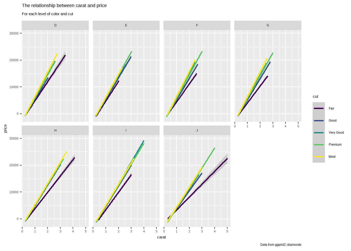
Figure C.14: Basic plot in default theme
Always start with a base theme, like theme_minimal() and set the size and font. Make sure to load any custom fonts.
font_add_google(name = "Nunito", family = "Nunito")
showtext_auto() # load the fonts

# set up custom theme to add to all plots
mytheme <- theme_minimal(     # always start with a base theme_****
  base_size = 16,             # 16-point font (adjusted for axes)
  base_family = "Nunito"      # custom font family
)
g + mytheme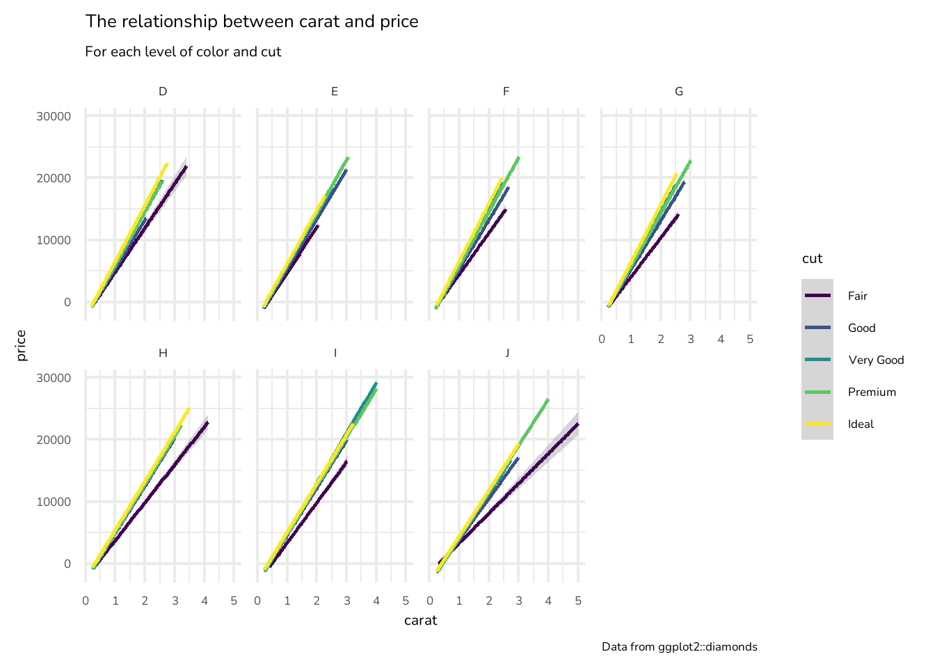
Figure C.15: Basic customised theme
Now add specific theme customisations. See ?theme for detailed explanations. Most theme arguments take a value of element_blank() to remove the feature entirely, or element_text(), element_line() or element_rect(), depending on whether the feature is text, a box, or a line.
# add more specific customisations with theme()
mytheme <- theme_minimal(
  base_size = 16,
  base_family = "Nunito"
) +
  theme(
    plot.background  = element_rect(fill = "black"),
    panel.background = element_rect(fill = "grey10",
                                    color = "grey30"),
    text             = element_text(color = "white"),
    strip.text       = element_text(hjust = 0), # left justify
    strip.background = element_rect(fill = "grey60", ),
    axis.text        = element_text(color = "grey60"),
    axis.line        = element_line(color = "grey60", size = 1),
    panel.grid       = element_blank(),
    plot.title       = element_text(hjust = 0.5), # center justify
    plot.subtitle    = element_text(hjust = 0.5, color = "grey60"),
    plot.caption     = element_text(face = "italic")
  )
g + mytheme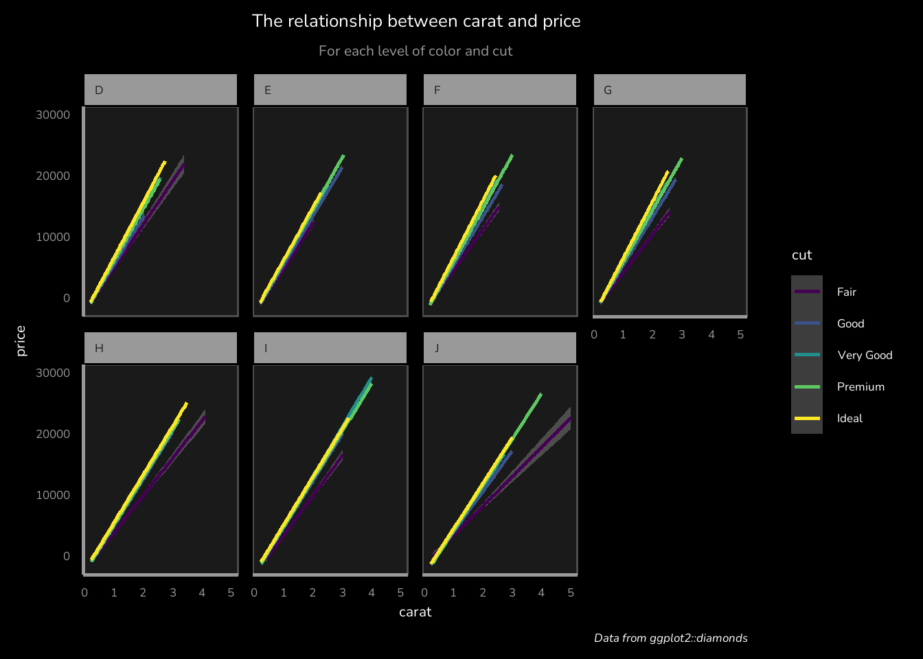
Figure C.16: Further customised theme
You can still add further theme customisation for specific plots.
g + mytheme +
  theme(
    legend.title      = element_text(size = 11),
    legend.text       = element_text(size = 9),
    legend.key.height = unit(0.2, "inches"),
    legend.position   = c(.9, 0.175)
  )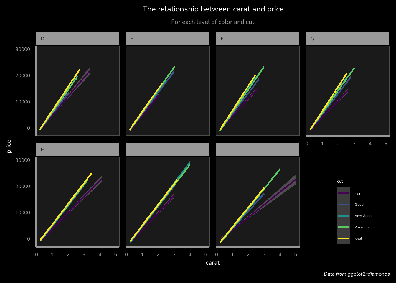
Figure C.17: Plot-specific customising.