H rtweet

H.0.1 Packages

In order to run these analyses you will need tidyverse for data wrangling,rtweet for getting the twitter data, tidytext for working with text, knitr for tidy tables, and igraph and ggraph for making pretty network plots.

In order to get data from Twitter you will need to have a twitter account and gain access to Twitter’s API. There are instructions for doing so here.

library(tidyverse)
library(knitr)
library(tidytext)
library(rtweet)
library(igraph)
library(ggraph)

H.0.2 Hashtag search

We can use rtweet to search for all tweets containing particular words or hashtags. It will return the last 18,000 tweets and only from the last 6-9 days. Be careful, there is a 15 minute time-out which means you can only retrieve 18,000 tweets every 15 minutes (there are various limits on what Twitter allows you to do with the data).

First, let’s search for all tweets that contain #GoT and #ForTheThrone.

There are various arguments to the search_tweets function, you can specify how many tweets you want to retrive with n, whether retweets should be included in the search results with include_rts and you can also specify the language of the user’s account with lang. Note that this doesn’t tell you what language the tweets are written in, only that the account language is set to e.g., English, so it’s not perfect. For additional options, see the help documentation.

tweets <- search_tweets(q = "#GoT OR #ForTheThrone", n = 18000, include_rts = FALSE, lang = "en")

H.0.3 Data wrangling

The output of search_tweets() is a list which makes it difficult to share. We need to do a little bit of tidying to turn it into a tibble, and additionally there’s a lot of data and we don’t need it all. I’m also going to add a tweet counter which will help when we move between wide and long-form. rtweet provides a huge amount of data, more than we’re going to use in this example so have a look through to see what you have access to - there are some great examples of how this data can be used here and here .

In the following code, I have added an identifier column tweet_number and then selected text (the actual text of the tweets), created_at (the timestamp of the tweet), source (iphone/android etc), followers_count (how many followers the accounts the tweets came from have), and country (like lang, the is the country specified on the account, not necessarily the country the tweeter is in).

dat <- tweets %>%
  mutate(tweet_number = row_number())%>%
  select(tweet_number, text, created_at, source, followers_count, country)%>%
  as_tibble()

You can download this file here so that you can reproduce my exact analyses (or you can use your own, but the results will look a bit different).

The first thing we need to do is tidy up the text by getting rid of punctuation, numbers, and links that aren’t of any interest to us. We can also remove the hashtags because we don’t want those to be included in any analysis. This code uses regular expressions which quite frankly make very little sense to me, I have copied and pasted this code from the Tidy Text book.

dat <- dat %>%
  mutate(text = str_replace_all(text, "[^\x01-\x7F]", ""),
         text = str_replace_all(text, "#GoT", ""),
         text = str_replace_all(text, "#ForTheThrone", ""),
         text = str_replace_all(text, "\\.|[[:digit:]]+", ""),
         text = str_replace_all(text, "https|amp|t.co", ""))

H.0.4 Time series

We can plot when the tweets were sent. This is somewhat uninteresting because it’s no longer airing, but it’s worth highlighting this as a feature. If you were watching live, you could use this to see the spikes in tweets when people are watching each episode live (different timezones will muddle this a little, you could filter by country perhaps).

ts_plot(tweets, by = "1 hours")

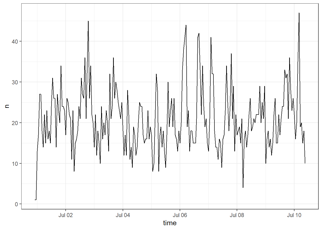
Figure H.1: Time series plot by hour

You can change the time interval with the by argument and you can also change the time zone. ts_plot creates a ggplot object so you can also add the usual ggplot layers to customise apperance.

ts_plot(tweets, by = "10 mins", tz = "GMT") +
  theme_minimal()+
  scale_y_continuous(name = "Number of tweets")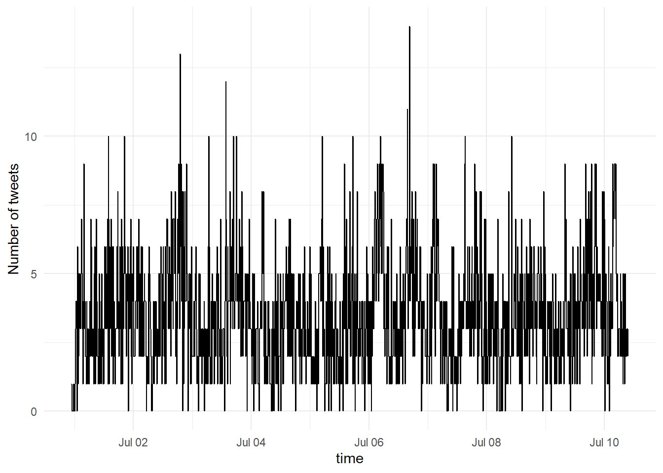

Figure H.2: Time series plot by 10 minute intervals

H.0.5 Tidy text and word frequencies

First, we can produce frequency plots for words used in all tweets to see which words are used most often in #GoT and #ForTheThrone tweets. To do this, we have to create a tidy dataset, just like we do when working with numerical data. We’re going to use the unnest_tokens function from tidytext which will separate each word on to a new line, something similar to like using gather (or pivot_longer as it will soon be known). Helpfully, this function will also convert all of our words to lower case which makes them a bit easier to work with.

The second part of the code removes all the stop words. Stop words are words that are commonly used but are of not real interest, for example function words like “the”, “a”, “it”. You can make your own list but tidytext helpfully comes with several databases. Look at the help documentation if you want to know more about these or change the defaults.

# create tidy text
dat_token <- dat %>%  
  unnest_tokens(word, text) %>%
  anti_join(stop_words, by = "word")

We can plot the 20 most frequent words used in all the tweets.

dat_token%>%
  na.omit()%>%
  count(word, sort = TRUE)%>%
  head(20) %>%
  mutate(word = reorder(word, n))%>%
  ggplot(aes(x = word, y = n))+
  geom_col()+
  coord_flip()

Figure H.3: Most frequent words

There’s quite a few words here that aren’t that helpful to us so it might be best to get rid of them (essentially we’re building our own list of stop words).

custom_stop <- c("gameofthrones", "hbo", "season", "game", "thrones", "lol", "tco", "https", "watch", "watching", "im", "amp")

dat_token <- dat_token %>%
  filter(!word %in% custom_stop)

Now we can try plotting the words again and make them pretty.

dat_token%>%
  na.omit()%>%
  count(word, sort = TRUE)%>%
  head(20) %>%
  mutate(word = reorder(word, n))%>%
  ggplot(aes(x = word, y = n, fill = word))+
  geom_col(show.legend = FALSE)+
  coord_flip()+
  scale_fill_viridis(discrete = TRUE)

Figure H.4: Most frequent words (edited)

To be honest, this isn’t that interesting because it’s so general, it might be more interesting to see how often each of the main characters are being mentioned.

One problem is that people on the internet are terrible at spelling and we need to have the exact spellings which means that for Daenerys, Jon, and Jaime, the chances that people will have spelled their names wrong is quite high (as my level 2 students who watched me live code the first version of this will attest) so first we’re going to correct those.

dat_token2 <- dat_token %>%
  mutate(word = recode(word, "khaleesi" = "daenerys",
                       "dany" = "daenerys",
                       "jamie" = "jaime",
                       "john" = "jon"))

characters <- c("jon", "daenerys", "bran", "arya", "sansa", "tyrion", "cersei", "jaime")

Now we can plot a count of how many times each name has been mentioned.

dat_token2 %>%
  filter(word %in% characters)%>%
  count(word, sort = TRUE) %>%
  mutate(word = reorder(word, n))%>%
  ggplot(aes(x = word, y = n, fill = word)) +
  geom_col(show.legend = FALSE) +
  coord_flip()+
  scale_y_continuous(name = "Number of mentions")+
  scale_x_discrete(name = "Character")+
  scale_fill_viridis(discrete = TRUE)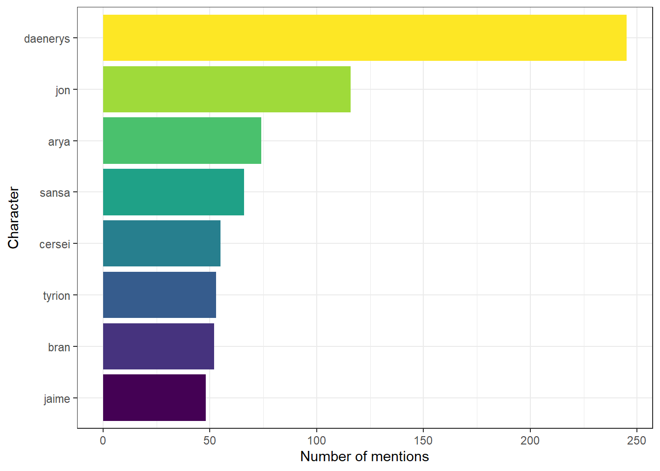

Figure H.5: Frequecy of mentions for each character

H.0.6 Bigram analysis

Rather than looking at individual words we can look at what words tend to co-occur. We want to use the data set where we’ve corrected the spelling so this is going to require us to transform from long to wide and then back to long because the night is dark and full of terror. DID YOU SEE WHAT I DID THERE.

dat_bigram <- dat_token2 %>%
  group_by(tweet_number) %>%  summarise(text = str_c(word, collapse = " "))%>% # this puts it back into wide-form
  unnest_tokens(bigram, text, token = "ngrams", n = 2, collapse = FALSE)%>% # and then this turns it into bigrams in a tidy format
  na.omit()

## `summarise()` ungrouping output (override with `.groups` argument)

dat_bigram %>%
  count(bigram, sort = TRUE)%>%
  head(10)%>%
  kable(align = "c")

bigram	n
freefolk gt	165
togive freefolk	164
se tvtime	103
watched episode	88
episode se	86
ice fire	85
song ice	81
jonsnow daenerys	73
bracelets fef	71
connected matter	71

Again there’s a bit of nonsense here and it’s a bit uninteresting but it’s worth highlighting this is something you can do. Now that we’ve got our bigrams we can plot these to see the connections between the different words. First, we’re going to use separate to put the two words into different columns, then we’ll count them up and plot them. If you want more information about this see the tidytext book online as I am entirely cribbing this from that book. The plot requires the packages igraph and ggraph.

bigrams_separated <- dat_bigram %>%
  separate(bigram, c("word1", "word2"), sep = " ")

# new bigram counts:
bigram_counts <- bigrams_separated %>% 
  count(word1, word2, sort = TRUE)

bigram_counts

# filter for only relatively common combinations (more than 20 occurances)
bigram_graph <- bigram_counts %>%
  filter(n > 20) %>%
  graph_from_data_frame()

# make a pretty network plot

ggraph(bigram_graph, layout = "fr") +
  geom_edge_link() +
  geom_node_point() +
  geom_node_text(aes(label = name), vjust = 1, hjust = 1)+
  theme_void()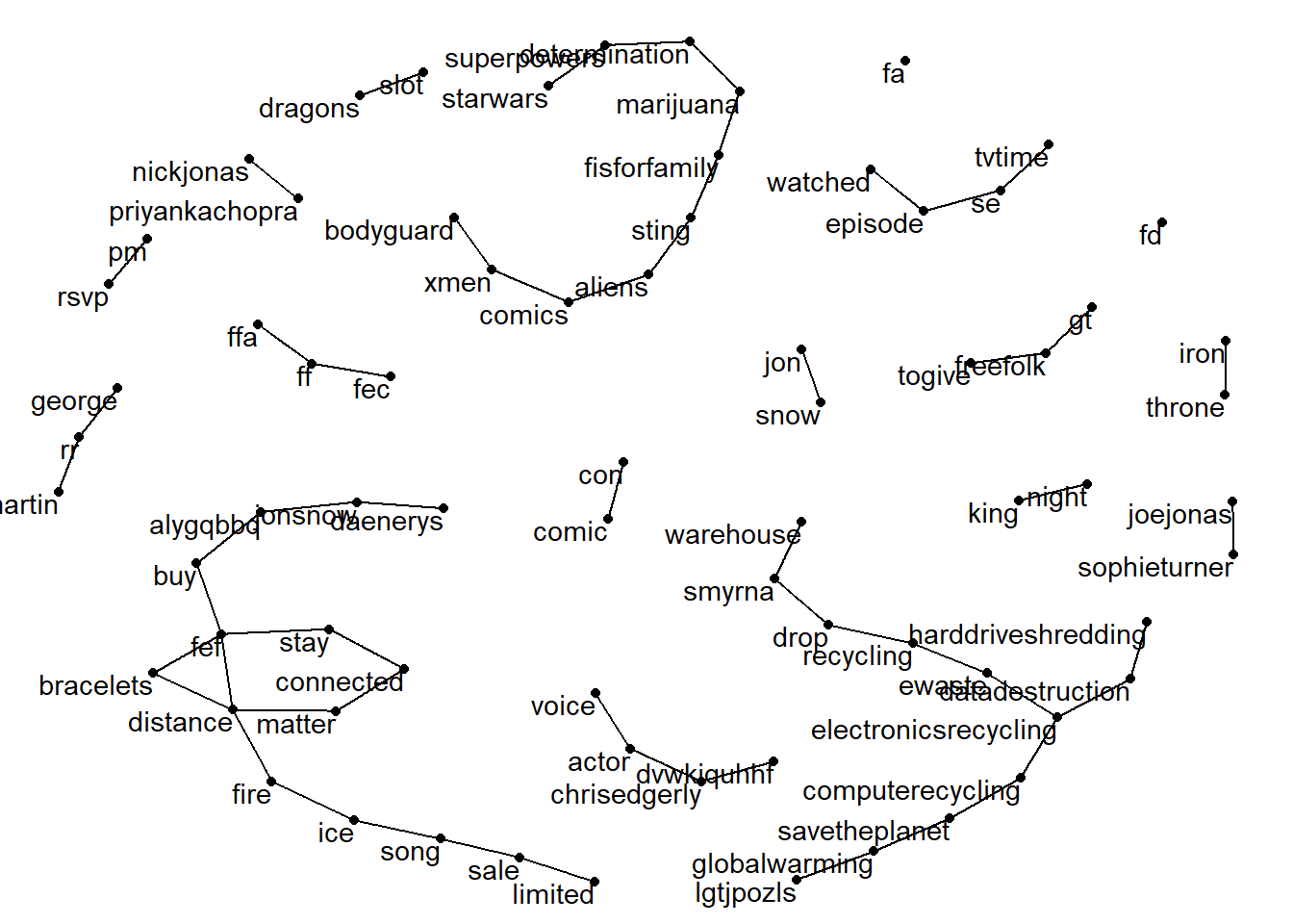

Figure H.6: Network graph of bigrams

## # A tibble: 30,134 x 3
##    word1     word2        n
##    <chr>     <chr>    <int>
##  1 freefolk  gt         165
##  2 togive    freefolk   164
##  3 se        tvtime     103
##  4 watched   episode     88
##  5 episode   se          86
##  6 ice       fire        85
##  7 song      ice         81
##  8 jonsnow   daenerys    73
##  9 bracelets fef         71
## 10 connected matter      71
## # ... with 30,124 more rows

I am still figuring out how to customise the aesthetics of ggraph.

H.0.7 Sentiment analysis

Sentiment analyses look at whether the expressed opinion in a bit of text is positive, negative, or neutral, using information from databases about the valance of different words. We can perform a sentiment analysis on the tweets that contain each character’s name to see whether e.g., Jon is mentioned in tweets that are largely positive or if Jaime is mentioned in tweets that are largely negative.

To do this, we first need to do a bit of wrangling. We’re going to transform it back to wide-form, then we’re going to add in in a column that says whether each character was mentioned in the tweet, then we’re going to transform it back to long-form.

dat_mentions <- dat_token2 %>%
  group_by(tweet_number) %>%
  summarise(text = str_c(word, collapse = " "))%>%
  mutate(jon = case_when(str_detect(text, ".jon") ~ TRUE, TRUE ~ FALSE),
         daenerys = case_when(str_detect(text, ".daenerys") ~ TRUE, TRUE ~ FALSE),
         bran = case_when(str_detect(text, ".bran") ~ TRUE, TRUE ~ FALSE),
         arya = case_when(str_detect(text, ".arya") ~ TRUE, TRUE ~ FALSE),
         sansa = case_when(str_detect(text, ".sansa") ~ TRUE, TRUE ~ FALSE),
         tyrion = case_when(str_detect(text, ".tyrion") ~ TRUE, TRUE ~ FALSE),
         cersei = case_when(str_detect(text, ".cersei") ~ TRUE, TRUE ~ FALSE),
         jaime = case_when(str_detect(text, ".jaime") ~ TRUE, TRUE ~ FALSE))%>%
  unnest_tokens(word, text) %>%
  anti_join(stop_words, by = "word")

## `summarise()` ungrouping output (override with `.groups` argument)

Once we’ve done this, we can then run a sentiment analysis on the tweets for each character. I still haven’t quite cracked iteration so this code is a bit repetitive, if you can give me the better way of doing this that’s less prone to copy and paste errors, please do.

jon <- dat_mentions %>%
  filter(jon)%>%
  inner_join(get_sentiments("bing"))%>%
  count(index = tweet_number, sentiment) %>%
  spread(sentiment, n, fill = 0) %>%
  mutate(sentiment = positive - negative)%>%
  mutate(character = "jon")

daenerys <- dat_mentions %>%
  filter(daenerys == "TRUE")%>%
  inner_join(get_sentiments("bing"))%>%
  count(index = tweet_number, sentiment) %>%
  spread(sentiment, n, fill = 0) %>%
  mutate(sentiment = positive - negative)%>%
  mutate(character = "daenerys")


bran <- dat_mentions %>%
  filter(bran == "TRUE")%>%
  inner_join(get_sentiments("bing"))%>%
  count(index = tweet_number, sentiment) %>%
  spread(sentiment, n, fill = 0) %>%
  mutate(sentiment = positive - negative)%>%
  mutate(character = "bran")

arya <- dat_mentions %>%
  filter(arya == "TRUE")%>%
  inner_join(get_sentiments("bing"))%>%
  count(index = tweet_number, sentiment) %>%
  spread(sentiment, n, fill = 0) %>%
  mutate(sentiment = positive - negative)%>%
  mutate(character = "arya")

sansa <- dat_mentions %>%
  filter(sansa == "TRUE")%>%
  inner_join(get_sentiments("bing"))%>%
  count(index = tweet_number, sentiment) %>%
  spread(sentiment, n, fill = 0) %>%
  mutate(sentiment = positive - negative)%>%
  mutate(character = "sansa")

tyrion <- dat_mentions %>%
  filter(tyrion == "TRUE")%>%
  inner_join(get_sentiments("bing"))%>%
  count(index = tweet_number, sentiment) %>%
  spread(sentiment, n, fill = 0) %>%
  mutate(sentiment = positive - negative)%>%
  mutate(character = "tyrion")

cersei <- dat_mentions %>%
  filter(cersei == "TRUE")%>%
  inner_join(get_sentiments("bing"))%>%
  count(index = tweet_number, sentiment) %>%
  spread(sentiment, n, fill = 0) %>%
  mutate(sentiment = positive - negative)%>%
  mutate(character = "cersei")

jaime <- dat_mentions %>%
  filter(jaime == "TRUE")%>%
  inner_join(get_sentiments("bing"))%>%
  count(index = tweet_number, sentiment) %>%
  spread(sentiment, n, fill = 0) %>%
  mutate(sentiment = positive - negative)%>%
  mutate(character = "jaime")


dat_sentiment <- bind_rows(jon,daenerys,bran,arya,sansa,tyrion,cersei,jaime) %>%
  group_by(character) %>%
  summarise(positive = sum(positive),
            negative = sum(negative),
            overall = sum(sentiment))%>%
  gather(positive:overall, key = type, value = score)%>%
  mutate(type = factor(type, levels = c("positive", "negative", "overall")))

Now that we’ve done all that we can display a table of positive, negative and overall sentiment scores. Bear in mind that not all words have an associated sentiment score, particularly if they’re a non-standard usage of English (as an aside, this makes RuPaul’s Drag Race very difficult to analyse because tidytext will think a sickening death drop is a bad thing).

dat_sentiment %>%
  spread(type, score)%>%
  arrange(desc(overall))%>%
  kable(align = "c")

character	positive	negative	overall
jaime	16	29	-13
tyrion	15	30	-15
sansa	26	44	-18
cersei	28	55	-27
arya	26	58	-32
bran	32	66	-34
daenerys	62	155	-93
jon	90	185	-95

Because there’s diferent numbers of tweets for each character, it might be more helpful to convert it to percentages to make it easier to compare.

dat_sentiment %>%
  spread(type, score)%>%
  group_by(character)%>%
  mutate(total = positive + negative)%>%
  mutate(positive_percent = positive/total*100,
         negative_percent = negative/total*100,
         sentiment = positive_percent - negative_percent)%>%
  select(character, positive_percent, negative_percent, sentiment)%>%
  arrange(desc(sentiment))%>%
  kable(align = "c")

character	positive_percent	negative_percent	sentiment
sansa	37.14286	62.85714	-25.71429
jaime	35.55556	64.44444	-28.88889
cersei	33.73494	66.26506	-32.53012
tyrion	33.33333	66.66667	-33.33333
jon	32.72727	67.27273	-34.54545
bran	32.65306	67.34694	-34.69388
arya	30.95238	69.04762	-38.09524
daenerys	28.57143	71.42857	-42.85714

They’re all quite negative because there’s no pleasing some people but there’s some face validity to the analysis given the order of the rankings. If you’d been watching this live you could have repeated this each episode to see how the reactions to the characters changes.

Let’s make that into a graph cause graphs are great.

dat_sentiment %>%
  spread(type, score)%>%
  group_by(character)%>%
  mutate(total = positive + negative)%>%
  mutate(positive_percent = positive/total*100,
         negative_percent = negative/total*100,
         sentiment = positive_percent - negative_percent)%>%
  select(character, positive_percent, negative_percent, sentiment)%>%
  arrange(desc(sentiment))%>%
  ggplot(aes(x = reorder(character,sentiment), y = sentiment)) +
  geom_col(show.legend = FALSE) +
  scale_y_continuous(name = "Overall sentiment (percent)")+
  scale_x_discrete(name = "Character")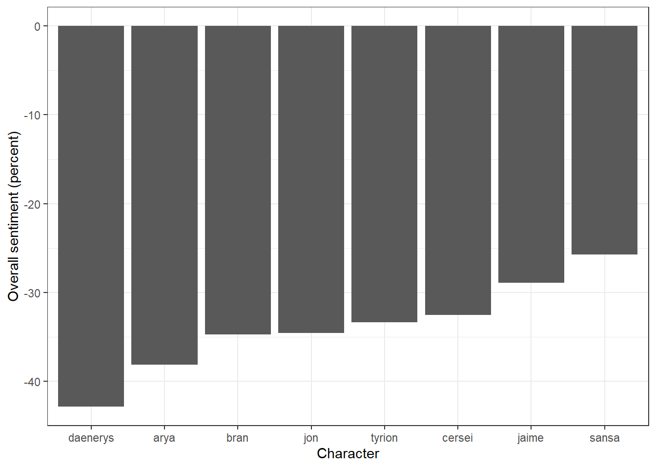

Figure H.7: Sentiment scores for each character

rtweet is such a cool package and I’ve found that the limits of what you can do with it are much more about one’s imagination. There’s much more you could do with this package but when I first ran these analyses I found that tracking RuPaul’s Drag Race was a fun way to learn a new package as it did give an insight into the fan reactions of one of my favourite shows. I also use this package to look at swearing on Twitter (replace the hashtags with swear words). The best way to learn what rtweet and tidytext can do for you is to find a topic you care about and explore the options it gives you. If you have any feedback on this tutorial you can find me on twitter: emilynordmann.