2 Reproducible Workflows
2.1 Learning Objectives
- Organise a project (video)
- Create and compile an Rmarkdown document (video)
- Edit the YAML header to add table of contents and other options
- Include a table
- Include a figure
- Report the output of an analysis using inline R
- Add a bibliography and citations
2.2 Setup
You will be given instructions in Section 2.4.4 below to set up a new project where you will keep all of your class notes. Section 2.5 gives instructions to set up an R Markdown script for this chapter.
For reference, here are the packages we will use in this chapter.
# packages needed for this chapter
library(tidyverse)  # various data manipulation functions
library(knitr)      # for table and image display
library(kableExtra) # for styling tables
library(papaja)     # for APA-style tables
library(gt)         # for fancy tables
library(DT)         # for interactive tables
Download the R Markdown Cheat Sheet.
2.3 Why use reproducible reports?
Have you ever worked on a report, creating a summary table for the demographics, making beautiful plots, getting the analysis just right, and copying all the relevant numbers into your manuscript, only to find out that you forgot to exclude a test run and have to redo everything?
A reproducible report fixes this problem. Although this requires a bit of extra effort at the start, it will more than pay you back by allowing you to update your entire report with the push of a button whenever anything changes.
Studies also show that many, if not most, papers in the scientific literature have reporting errors. For example, more than half of over 250,000 psychology papers published between 1985 and 2013 have at least one value that is statistically incompatible, such as a p-value that is not possible given a t-value and degrees of freedom (Nuijten et al., 2016). Reproducible reports help avoid transcription and rounding errors.
We will make reproducible reports following the principles of literate programming. The basic idea is to have the text of the report together in a single document along with the code needed to perform all analyses and generate the tables. The report is then "compiled" from the original format into some other, more portable format, such as HTML or PDF. This is different from traditional cutting and pasting approaches where, for instance, you create a graph in Microsoft Excel or a statistics program like SPSS and then paste it into Microsoft Word.
2.4 Organising a project
First, we need to get organised. Projects in RStudio are a way to group all of the files you need for one project. Most projects include scripts, data files, and output files like the PDF report created by the script or images.
2.4.1 File System
Modern computers tend to hide the file system from users, but we need to understand a little bit about how files are stored on your computer in order to get a script to find your data. Your computer's file system is like a big box (or directory) that contains both files and smaller boxes, or "subdirectories". You can specify the location of a file with its name and the names of all the directories it is inside.
For example, if Lisa is looking for a file called report.Rmdon their Desktop, they can specify the full file path like this: /Users/lisad/Desktop/report.Rmd, because the Desktop directory is inside the lisad directory, which is inside the Users directory, which is located at the base of the whole file system. If that file was on your desktop, you would probably have a different path unless your user directory is also called lisad. You can also use the ~ shortcut to represent the user directory of the person who is currently logged in, like this: ~/Desktop/report.Rmd.
2.4.2 Working Directory
Where should you put all of your files? You usually want to have all of your scripts and data files for a single project inside one folder on your computer, the working directory for that project. You can organise files in subdirectories inside this main project directory, such as putting all raw data files in a directory called data and saving any image files to a directory called images.
Your script should only reference files in three types of locations, using the appropriate format.
| Where | Example |
|---|---|
| on the web | "https://psyteachr.github.io/reprores-v3/data/5factor.xlsx" |
| in the working directory | "5factor.xlsx" |
| in a subdirectory | "data/5factor.xlsx" |
Never set or change your working directory in a script.
R Markdown files will automatically use the same directory the .Rmd file is in as the working directory.
If your script needs a file in a subdirectory of your working directory, such as, data/5factor.xlsx, load it in using a relative path so that it is accessible if you move the working directory to another location or computer:
dat <- read_csv("data/5factor.xlsx") # correctDo not load it in using an absolute path:
dat <- read_csv("C:/My Files/2020-2021/data/5factor.xlsx") # wrongAlso note the convention of using forward slashes, unlike the Windows-specific convention of using backward slashes. This is to make references to files work for everyone, regardless of their operating system.
2.4.3 Naming Things
Name files so that both people and computers can easily find things. Here are some important principles:
- file and directory names should only contain letters, numbers, dashes, and underscores, with a full stop (
.) between the file name and extension (that means no spaces!) - be consistent with capitalisation (set a rule to make it easy to remember, like always use lowercase)
- use underscores (
_) to separate parts of the file name, and dashes (-) to separate words in a section - name files with a pattern that alphabetises in a sensible order and makes it easy for you to find the file you're looking for
- prefix a filename with an underscore to move it to the top of the list, or prefix all files with numbers to control their order
- use YYYY-MM-DD format for dates so they sort in chronological order
For example, these file names are a mess:
Data (Participants) 11-15.xlsfinal report2.docParticipants Data Nov 12.xlsproject notes.txtQuestionnaire Data November 15.xlsreport.docreport final.doc
Here is one way to structure them so that similar files have the same structure and it's easy for a human to scan the list or to use code to find relevant files. See if you can figure out what the missing one should be.
_project-notes.txtdata_participants_2021-11-12.xlsdata_participants_2021-11-15.xlsreport_v1.docreport_v2.docreport_v3.doc
Think of other ways to name the files above. Look at some of your own project files and see what you can improve.
2.4.4 Start a Project
Now that we understand how the file system work and how to name things to make it easier for scripts to access them, we're ready to make our class project.
First, make a new directory where you will keep all of your materials for this class (I called mine reprores-2022). You can set this directory to be the default working directory under the General tab of the Global Options. This means that files will be saved here by default if you aren't working in a project.
It can sometimes cause problems if this directory is in OneDrive or if the full file path has special characters or is more than 260 characters on some Windows machines.
Next, choose New Project... under the File menu to create a new project called reprores-class-notes. Make sure you save it inside the directory you just made. RStudio will restart itself and open with this new project directory as the working directory.
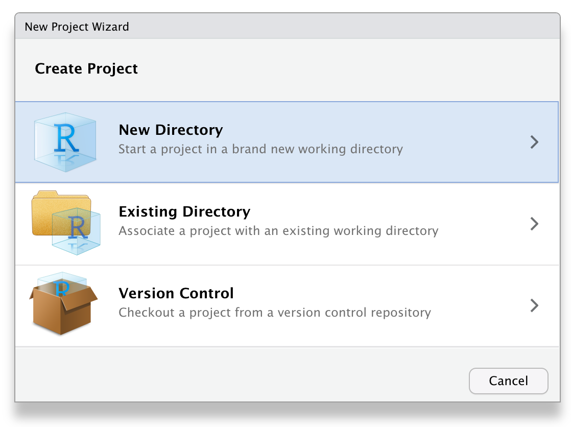
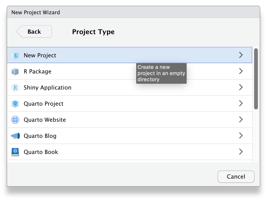
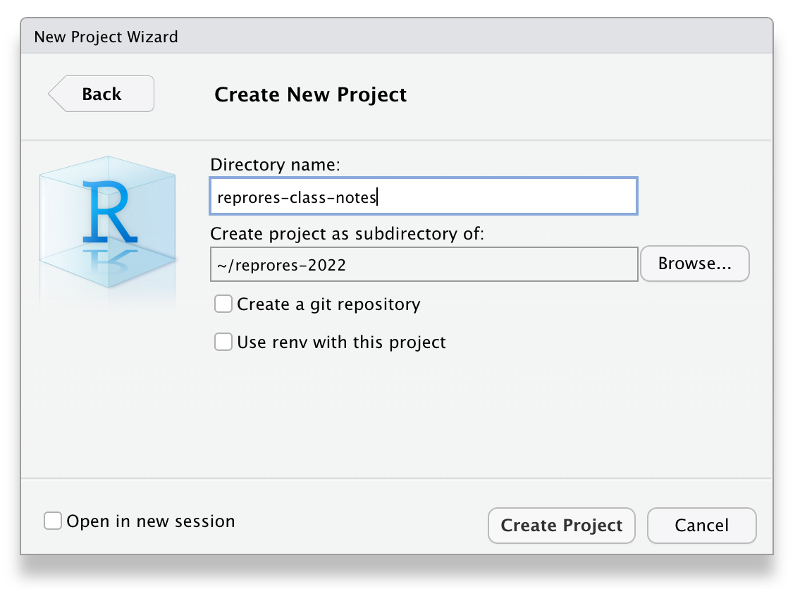
Figure 2.1: Starting a new project.
Click on the Files tab in the lower right pane to see the contents of the project directory. You will see a file called reprores-class-notes.Rproj, which is a file that contains all of the project information.You can double-click on it to open up the project.
Depending on your settings, you may also see a directory called .Rproj.user, which contains your specific user settings. You can ignore this and other "invisible" files that start with a full stop.
2.5 R Markdown
In this lesson, we will learn to make an R Markdown document with a table of contents, appropriate headers, code chunks, tables, images, inline R, and a bibliography.
There is a new type of reproducible report format called quarto that is very similar to R Markdown. We won't be using quarto in this class because it has a few small differences that get confusing if you're learning both quarto and R Markdown at the same time, but you should be able to pick up quarto very easily once you've learned R Markdown.
We will use R Markdown to create reproducible reports, which enables mixing of text and code. A reproducible script will contain sections of code in code blocks. A code block starts and ends with three backtick symbols in a row, with some information about the code between curly brackets, such as {r chunk-name, echo=FALSE} (this runs the code, but does not show the text of the code block in the compiled document). The text outside of code blocks is written in markdown, which is a way to specify formatting, such as headers, paragraphs, lists, bolding, and links.
---
title: "Reproducible Script"
author: "Lisa DeBruine"
output: html_document
---

```{r setup, include=FALSE}
knitr::opts_chunk$set(echo = TRUE)
library(tidyverse)
```

## Simulate Data

Here we will simulate data from a study with two conditions.
The mean in condition A is 0 and the mean in condition B is 1.

```{r simulate}
n <- 100

data <- data.frame(
  id = 1:n,
  condition = c("A", "B") |> rep(each = n/2),
  dv = c(rnorm(n/2, 0), rnorm(n/2, 1))
)
```

## Plot Data

```{r condition-plot, echo = FALSE}
ggplot(data, aes(condition, dv)) +
  geom_violin(trim = FALSE) +
  geom_boxplot(width = 0.25,
               aes(fill = condition),
               show.legend = FALSE)
```
If you open up a new R Markdown file from a template, you will see an example document with several code blocks in it. To create an HTML or PDF report from an R Markdown (Rmd) document, you compile it. Compiling a document is called knitting in RStudio. There is a button that looks like a ball of yarn with needles through it that you click on to compile your file into a report.
Create a new R Markdown file from the File > New File > R Markdown... menu. Change the title and author, save the file as 02-repro.Rmd, then click the knit button to create an html file.
2.5.1 YAML Header
The YAML header is where you can set several options.
---
title: "My Demo Document"
author: "Me"
output:
  html_document:
    toc: true
    toc_float:
      collapsed: false
      smooth_scroll: false
    number_sections: false
---
Try changing the values from false to true to see what the options do.
The df_print: kable option prints data frames using knitr::kable. You'll learn below how to further customise tables.
The built-in bootswatch themes are: default, cerulean, cosmo, darkly, flatly, journal, lumen, paper, readable, sandstone, simplex, spacelab, united, and yeti. You can view and download more themes.
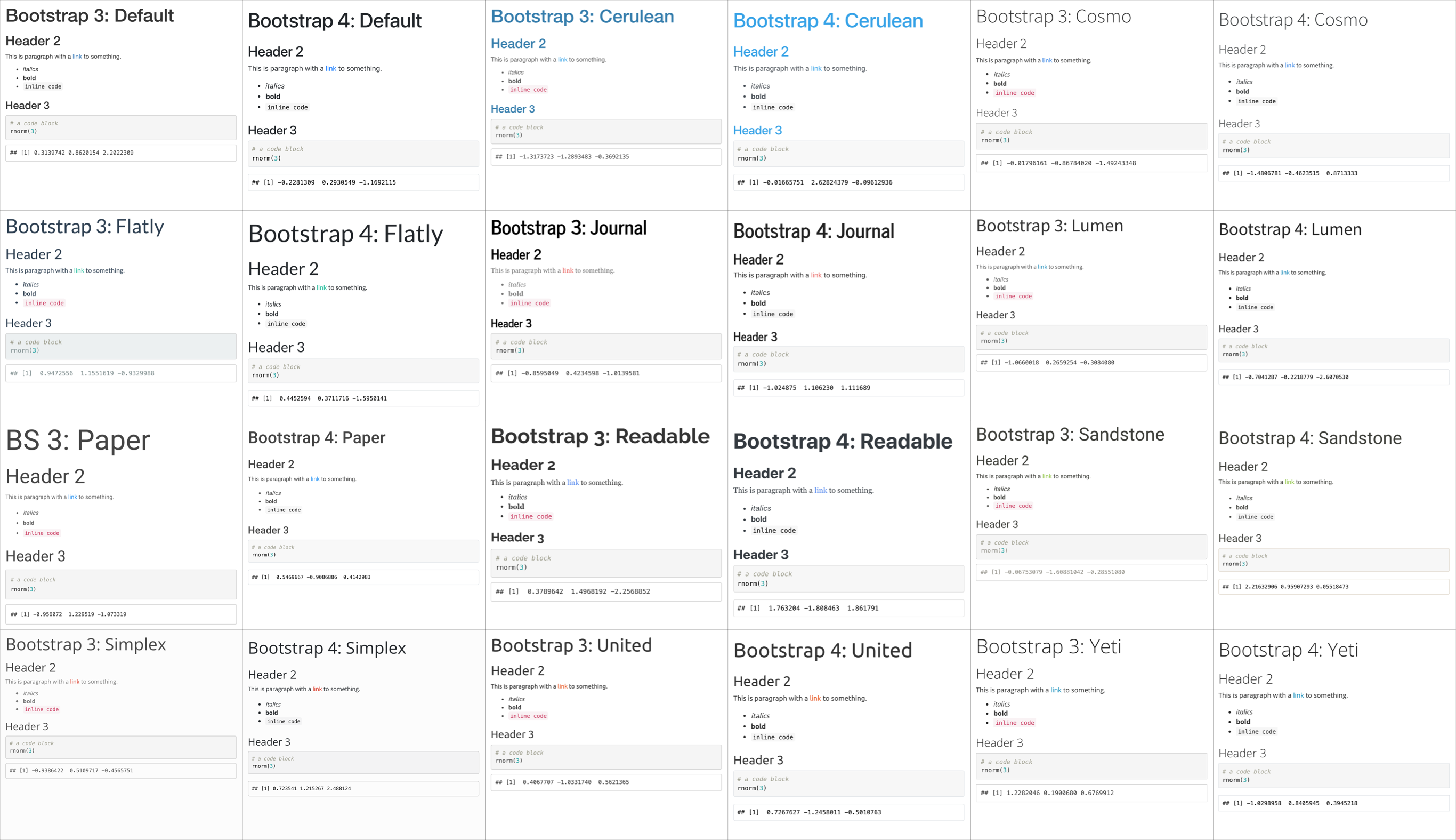
Figure 2.2: Light themes in versions 3 and 4.
2.5.2 Setup
When you create a new R Markdown file in RStudio using the default template, a setup chunk is automatically created.
You can set more default options for code chunks here. See the knitr options documentation for explanations of the possible options.
```{r setup, include=FALSE}
knitr::opts_chunk$set(
  fig.width  = 8,
  fig.height = 5,
  fig.path   = 'images/',
  echo       = FALSE,
  warning    = TRUE,
  message    = FALSE,
  cache      = FALSE
)```The code above sets the following options:
-
fig.width = 8: default figure width is 8 inches (you can change this for individual figures) -
fig.height = 5: default figure height is 5 inches -
fig.path = 'images/': figures are saved in the directory "images" -
echo = FALSE: do not show code chunks in the rendered document -
warning = FALSE: do not show any function warnings -
message = FALSE: do not show any function messages -
cache = FALSE: run all the code to create all of the images and objects each time you knit (set toTRUEif you have time-consuming code)
Find a list of the current chunk options by typing str(knitr::opts_chunk$get()) in the console.
You can also add the packages you need in this chunk using library(). Often when you are working on a script, you will realize that you need to load another add-on package. Don't bury the call to library(package_I_need) way down in the script. Put it in the top, so the user has an overview of what packages are needed.
We'll be using function from the package tidyverse, so load that in your setup chunk.
2.5.3 Structure
If you include a table of contents (toc), it is created from your document headers. Headers in markdown are created by prefacing the header title with one or more hashes (#).
Use the following structure when developing your own analysis scripts:
- load in any add-on packages you need to use
- define any custom functions
- load or simulate the data you will be working with
- work with the data
- save anything you need to save
Delete the default text and add some structure to your document by creating headers and subheaders. We're going to load some data, create a summary table, plot the data, and analyse it.
2.5.4 Code Chunks
You can include code chunks that create and display images, tables, or computations to include in your text. Let's start by loading some data.
First, create a code chunk in your document. This code loads some data from the web.
pets <- read_csv("https://psyteachr.github.io/reprores/data/pets.csv",
show_col_types = FALSE)2.5.6 In-line R
Now let's analyse the pets data to see if cats are heavier than ferrets. First we'll run the analysis code. Then we'll save any numbers we might want to use in our manuscript to variables and round them appropriately. Finally, we'll use glue::glue() to format a results string.
# analysis
cat_weight <- filter(pets, pet == "cat") %>% pull(weight)
ferret_weight <- filter(pets, pet == "ferret") %>% pull(weight)
weight_test <- t.test(cat_weight, ferret_weight)

# round individual values you want to report
t <- weight_test$statistic %>% round(2)
df <- weight_test$parameter %>% round(1)
p <- weight_test$p.value %>% round(3)
# handle p-values < .001
p_symbol <- ifelse(p < .001, "<", "=")
if (p < .001) p <- .001

# format the results string
weight_result <- glue::glue("t = {t}, df = {df}, p {p_symbol} {p}")
You can insert the results into a paragraph with inline R code that looks like this:
Cats were significantly heavier than ferrets (`r weight_result`).Rendered text:
Cats were significantly heavier than ferrets (t = 18.42, df = 180.4, p < 0.001).
2.5.7 Tables
Next, create a code chunk where you want to display a table of the descriptives (e.g., Participants section of the Methods). We'll use tidyverse functions you will learn in the data wrangling lectures to create summary statistics for each group.
summary_table <- pets %>%
  group_by(pet) %>%
  summarise(
    n = n(),
    mean_weight = mean(weight),
    mean_score = mean(score)
  )

# print
summary_table| pet | n | mean_weight | mean_score |
|---|---|---|---|
| cat | 300 | 9.371613 | 90.23667 |
| dog | 400 | 19.067974 | 99.98250 |
| ferret | 100 | 4.781569 | 111.78000 |
The table above will print in tibble format in the interactive view, but will use the format from the df_print setting in the YAML header when you knit.
The table above is OK, but it could be more reader-friendly by changing the column labels, rounding the means, and adding a caption. You can use knitr::kable() for this, or more specialised functions from other packages to format your tables.
newnames <- c("Pet Type", "N", "Mean Weight", "Mean Score")

knitr::kable(summary_table,
             digits = 2,
             col.names = newnames,
caption = "Summary statistics for the pets dataset.")| Pet Type | N | Mean Weight | Mean Score |
|---|---|---|---|
| cat | 300 | 9.37 | 90.24 |
| dog | 400 | 19.07 | 99.98 |
| ferret | 100 | 4.78 | 111.78 |
The kableExtra package gives you a lot of flexibility with table display.
library(kableExtra)

kable(summary_table,
      digits = 2,
      col.names = c("Pet Type", "N", "Weight", "Score"),
      caption = "Summary statistics for the pets dataset.") |>
  kable_classic() |>
  kable_styling(full_width = FALSE, font_size = 20) |>
  add_header_above(c(" " = 2, "Means" = 2)) |>
kableExtra::row_spec(2, bold = TRUE, background = "lightyellow")|
Means
|
|||
|---|---|---|---|
| Pet Type | N | Weight | Score |
| cat | 300 | 9.37 | 90.24 |
| dog | 400 | 19.07 | 99.98 |
| ferret | 100 | 4.78 | 111.78 |
papaja helps you create APA-formatted manuscripts, including tables.
papaja::apa_table(summary_table,
                  col.names = c("Pet Type", "N", "Weight", "Score"),
                  caption = "Summary statistics for the pets dataset.",
col_spanners = list("Means" = c(3, 4)))| Pet Type | N | Weight | Score |
|---|---|---|---|
| cat | 300 | 9.37 | 90.24 |
| dog | 400 | 19.07 | 99.98 |
| ferret | 100 | 4.78 | 111.78 |
The gt package allows for even more customisation.
library(gt)

gt(summary_table, caption = "Summary statistics for the pets dataset.") |>
  fmt_number(columns = c(mean_weight, mean_score),
            decimals = 2) |>
  cols_label(pet = "Pet Type",
             n = "N",
             mean_weight = "Weight",
             mean_score = "Score") |>
  tab_spanner(label = "Means",
              columns = c(mean_weight, mean_score)) |>
opt_stylize(style = 6, color = "blue")| Pet Type | N | Means | |
|---|---|---|---|
| Weight | Score | ||
| cat | 300 | 9.37 | 90.24 |
| dog | 400 | 19.07 | 99.98 |
| ferret | 100 | 4.78 | 111.78 |
2.5.8 Images
Next, create a code chunk where you want to display an image in your document. Let's put it in the Results section. We'll use some code that you'll learn more about in the data visualisation lecture to show violin-boxplots for the groups.
Notice how the figure caption is formatted in the chunk options.
```{r pet-plot, fig.cap="Figure 1. Scores by pet type and country."}
ggplot(pets, aes(pet, score, fill = country)) +
  geom_violin(alpha = 0.5) +
  geom_boxplot(width = 0.25,
               position = position_dodge(width = 0.9),
               show.legend = FALSE) +
  scale_fill_manual(values = c("orange", "dodgerblue")) +
  labs(x = "", y = "Score") +
  theme(text = element_text(size = 20, family = "Times"))
```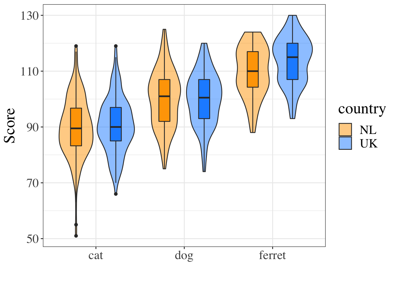
Figure 2.3: Figure 1. Scores by pet type and country.
The last line changes the default text size and font, which can be useful for generating figures that meet a journal's requirements.
You can also include images that you did not create in R using the typical markdown syntax for images:
](images/memes/x-all-the-things.png){style="width: 50%"}
All the Things by Hyperbole and a Half
2.5.9 Linked documents
If you need to create longer reports with links between sections, you can edit the YAML to use an output format from the bookdown package. bookdown::html_document2 is a useful one that adds figure and table numbers automatically to any figures or tables with a caption and allows you to link to these by reference.
To create links to tables and figures, you need to name the code chunk that created your figures or tables, and then call those names in your inline coding:
```{r my-table}
# table code here``````{r my-figure}
# figure code here```See Table\ \@ref(tab:my-table) or Figure\ \@ref(fig:my-figure).The code chunk names can only contain letters, numbers and dashes. If they contain other characters like spaces or underscores, the referencing will not work.
You can also link to different sections of your report by naming your headings with {#}:
# My first heading {#heading-1}

## My second heading {#heading-2}

See Section\ \@ref(heading-1) and Section\ \@ref(heading-2)
The code below shows how to link text to figures or tables in a full report using the built-in diamonds dataset - use your reports.Rmd to create this document now. You can see the HTML output here.
---
title: "Linked Document Demo"
output:
  bookdown::html_document2:
    number_sections: true
---

```{r setup, include=FALSE}
knitr::opts_chunk$set(echo = FALSE,
                      message = FALSE,
                      warning = FALSE)
library(tidyverse)
library(kableExtra)
theme_set(theme_minimal())
```

Diamond price depends on many features, such as:

- cut (See Table\ \@ref(tab:by-cut))
- colour (See Table\ \@ref(tab:by-colour))
- clarity (See Figure\ \@ref(fig:by-clarity))
- carats (See Figure\ \@ref(fig:by-carat))
- See section\ \@ref(conclusion) for concluding remarks

## Tables

### Cut

```{r by-cut}
diamonds %>%
  group_by(cut) %>%
  summarise(avg = mean(price),
            .groups = "drop") %>%
  kable(digits = 0,
        col.names = c("Cut", "Average Price"),
        caption = "Mean diamond price by cut.") %>%
  kable_material()
```

### Colour

```{r by-colour}
diamonds %>%
  group_by(color) %>%
  summarise(avg = mean(price),
            .groups = "drop") %>%
  kable(digits = 0,
        col.names = c("Cut", "Average Price"),
        caption = "Mean diamond price by colour.") %>%
  kable_material()
```

## Plots

### Clarity

```{r by-clarity, fig.cap = "Diamond price by clarity"}
ggplot(diamonds, aes(x = clarity, y = price)) +
  geom_boxplot()
```

### Carats

```{r by-carat, fig.cap = "Diamond price by carat"}
ggplot(diamonds, aes(x = carat, y = price)) +
  stat_smooth()
```

### Concluding remarks {#conclusion}

I am not rich enough to worry about any of this.
This format defaults to numbered sections, so set number_sections: false in the YAML header if you don't want this. If you remove numbered sections, links like \@ref(conclusion) will show "??", so you need to use URL link syntax instead, like this:
See the [last section](#conclusion) for concluding remarks.2.6 Bibliography
There are several ways to do in-text references and automatically generate a bibliography in R Markdown. Markdown files need to link to a BibTex or JSON file (a plain text file with references in a specific format) that contains the references you need to cite. You specify the name of this file in the YAML header, like bibliography: refs.bib and cite references in text using an at symbol and a shortname, like [@tidyverse]. You can also include a Citation Style Language (.csl) file to format your references in, for example, APA style.
---
title: "My Paper"
author: "Me"
output:
  html_document:
    toc: true
bibliography: refs.bib
csl: apa.csl
2.6.1 Converting from reference software
Most reference software like EndNote or Zotero has exporting options that can export to BibTeX format. You just need to check the shortnames in the resulting file.
Please start using a reference manager consistently through your research career. It will make your life so much easier. Zotero is probably the best one.
- If you don't already have one, set up a Zotero account
- Add the connector for your web browser (if you're on a computer you can add browser extensions to)
- Navigate to Easing Into Open Science and add this reference to your library with the browser connector
- Go to your library and make a new collection called "Open Research" (click on the + icon after
My Library)
- Drag the reference to Easing Into Open Science into this collection
- Export this collection as BibTex
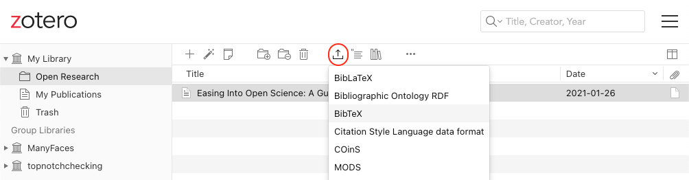
Figure 2.4: Export a bibliography file from Zotero
The exported file should look like this:
@article{kathawalla_easing_2021,
    title = {Easing {Into} {Open} {Science}: {A} {Guide} for {Graduate} {Students} and {Their} {Advisors}},
    volume = {7},
    issn = {2474-7394},
    shorttitle = {Easing {Into} {Open} {Science}},
    url = {https://doi.org/10.1525/collabra.18684},
    doi = {10.1525/collabra.18684},
    abstract = {This article provides a roadmap to assist graduate students and their advisors to engage in open science practices. We suggest eight open science practices that novice graduate students could begin adopting today. The topics we cover include journal clubs, project workflow, preprints, reproducible code, data sharing, transparent writing, preregistration, and registered reports. To address concerns about not knowing how to engage in open science practices, we provide a difficulty rating of each behavior (easy, medium, difficult), present them in order of suggested adoption, and follow the format of what, why, how, and worries. We give graduate students ideas on how to approach conversations with their advisors/collaborators, ideas on how to integrate open science practices within the graduate school framework, and specific resources on how to engage with each behavior. We emphasize that engaging in open science behaviors need not be an all or nothing approach, but rather graduate students can engage with any number of the behaviors outlined.},
    number = {1},
    urldate = {2022-09-07},
    journal = {Collabra: Psychology},
    author = {Kathawalla, Ummul-Kiram and Silverstein, Priya and Syed, Moin},
    month = jan,
    year = {2021},
    pages = {18684},
}
2.6.2 Creating a BibTeX File
You can also add references manually. In RStudio, go to File > New File... > Text File and save the file as "refs.bib".
Next, add the line bibliography: refs.bib to your YAML header.
2.6.3 Adding references
You can add references to a journal article in the following format:
@article{shortname,
  author = {Author One and Author Two and Author Three},
  title = {Paper Title},
  journal = {Journal Title},
  volume = {vol},
  number = {issue},
  pages = {startpage--endpage},
  year = {year},
  doi = {doi}
}
See A complete guide to the BibTeX format for instructions on citing books, technical reports, and more.
You can get the reference for an R package using the functions citation() and toBibtex(). You can paste the bibtex entry into your bibliography.bib file. Make sure to add a short name (e.g., "ggplot2") before the first comma to refer to the reference.
## @Book{,
##   author = {Hadley Wickham},
##   title = {ggplot2: Elegant Graphics for Data Analysis},
##   publisher = {Springer-Verlag New York},
##   year = {2016},
##   isbn = {978-3-319-24277-4},
##   url = {https://ggplot2.tidyverse.org},
## }
Google Scholar entries have a BibTeX citation option. This is usually the easiest way to get the relevant values if you can't add a citation through the Zotero browser connector, although you have to add the DOI yourself. You can keep the suggested shortname or change it to something that makes more sense to you.
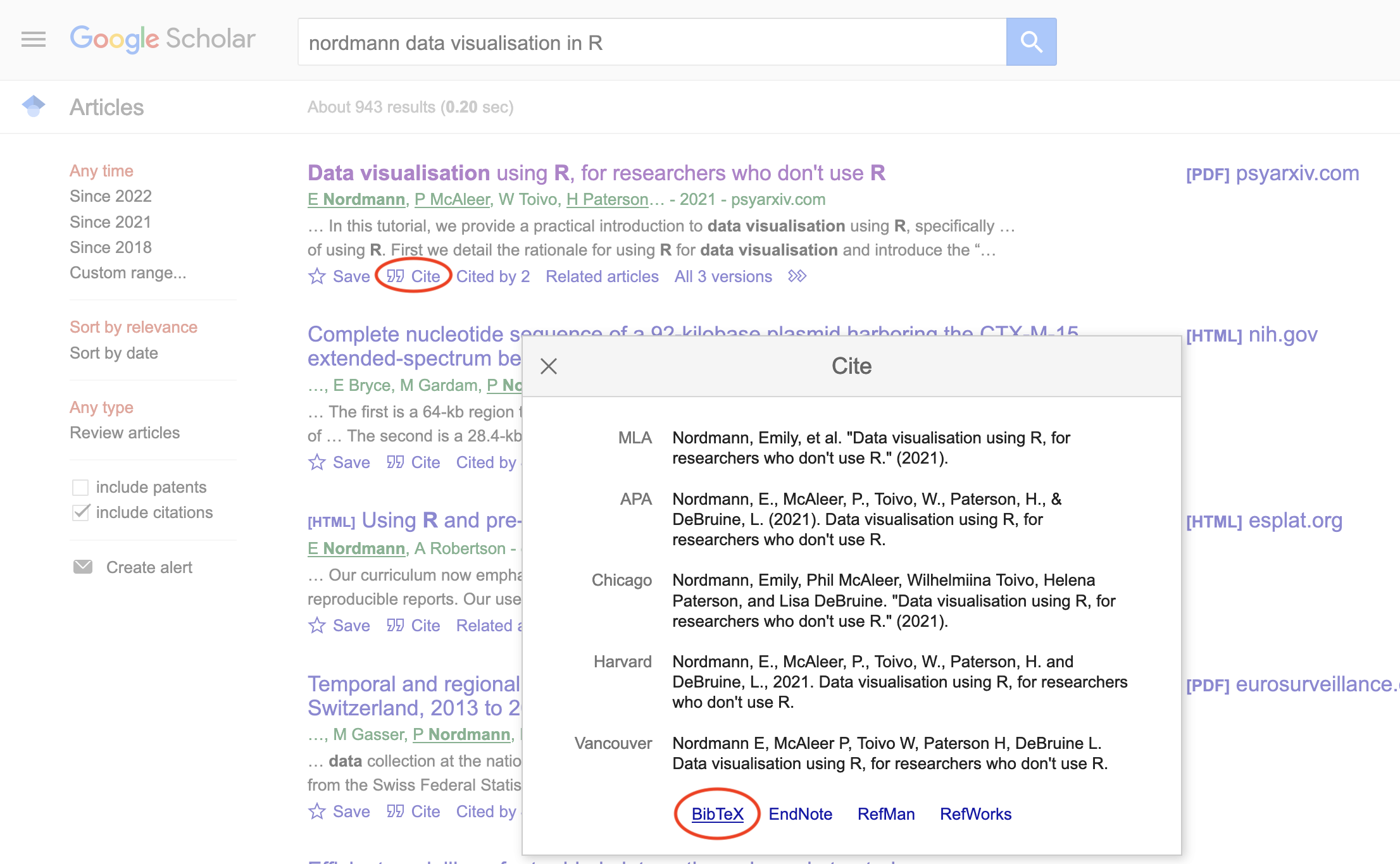
Figure 2.5: Get BibTex citations from Google Scholar.
2.6.4 Citing references
You can cite references in text like this:
This tutorial uses several R packages [@tidyverse;@rmarkdown].This tutorial uses several R packages (Allaire et al., 2018; Wickham, 2017).
Put a minus in front of the @ if you just want the year:
Kathawalla and colleagues [-@kathawalla_easing_2021] explain how to introduce open research practices into your postgraduate studies.Kathawalla and colleagues (2021) explain how to introduce open research practices into your postgraduate studies.
2.6.5 Uncited references
If you want to add an item to the reference section without citing, it, add it to the YAML header like this:
nocite: |
  @kathawalla_easing_2021, @broman2018data, @nordmann2022data
Or add all of the items in the .bib file like this:
nocite: '@*'2.6.6 Citation Styles
You can search a list of style files for various journals and download a file that will format your bibliography for a specific journal's style. You'll need to add the line csl: filename.csl to your YAML header.
Add some citations to your refs.bib file, reference them in your text, and render your manuscript to see the automatically generated reference section. Try a few different citation style files.
2.6.7 Reference Section
By default, the reference section is added to the end of the document. If you want to change the position (e.g., to add figures and tables after the references), include <div id="refs"></div> where you want the references.
Add in-text citations and a reference list to your report.
2.7 Custom Templates
Some packages provide custom R Markdown templates. reprores has a Report template that shows all of the possible options in the YAML header, has bibliography and style files, and explains how to set up linked figures and tables. Because it contains multiple files, RStudio will ask you to create a new folder to keep all of the files in.
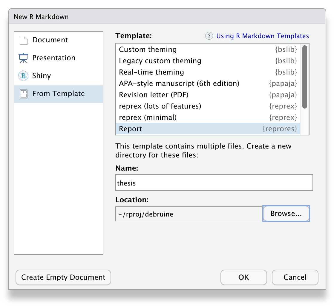
Figure 2.6: The custom R markdown template from reprores.
Start a report with the Report template and knit it. Try changing or deleting options.
2.8 Glossary
| term | definition |
|---|---|
| absolute path | A file path that starts with / and is not appended to the working directory |
| chunk | A section of code in an R Markdown file |
| directory | A collection or "folder" of files on a computer. |
| extension | The end part of a file name that tells you what type of file it is (e.g., .R or .Rmd). |
| knit | To create an HTML, PDF, or Word document from an R Markdown (Rmd) document |
| markdown | A way to specify formatting, such as headers, paragraphs, lists, bolding, and links. |
| path | A string representing the location of a file or directory. |
| project | A way to organise related files in RStudio |
| r markdown | The R-specific version of markdown: a way to specify formatting, such as headers, paragraphs, lists, bolding, and links, as well as code blocks and inline code. |
| relative path | The location of a file in relation to the working directory. |
| reproducibility | The extent to which the findings of a study can be repeated in some other context |
| working directory | The filepath where R is currently reading and writing files. |
| yaml | A structured format for information |
2.9 Further Resources
- Chapter 27: R Markdown in R for Data Science
- R Markdown Cheat Sheet
- R Markdown reference Guide
- R Markdown Tutorial
- R Markdown: The Definitive Guide by Yihui Xie, J. J. Allaire, & Garrett Grolemund
- Project Structure by Danielle Navarro
- How to name files by Jenny Bryan
- Papaja Reproducible APA Manuscripts
- The Turing Way
2.5.5 Comments
You can add comments inside R chunks with the hash symbol (
#). The R interpreter will ignore characters from the hash to the end of the line.It's usually good practice to start a code chunk with a comment that explains what you're doing there, especially if the code is not explained in the text of the report.
If you name your objects clearly, you often don't need to add clarifying comments. For example, if I'd named the three objects above
total_pet_n,mean_scoreandsd_score, I would omit the comments.Another use for comments is to "comment out" a section of code that you don't want to run, but also don't want to delete. For example, you might include the code used to install a package in your script, but you should always comment it out so the script doesn't force a lengthy installation every time it's run.
You can comment or uncomment multiple lines at once by selecting the lines and typing Cmd-shift-C (Mac) or Ctrl-shift-C (Windows).
It's a bit of an art to comment your code well. The best way to develop this skill is to read a lot of other people's code and have others review your code.