6 Chi-square and one-sample t-test
Intended Learning Outcomes
By the end of this chapter you should be able to:
- compute a Cross-tabulation Chi-square test and report the results
- compute a one-sample t-test and report the results
- understand when to use a non-parametric equivalent for the one-sample t-test, compute it, and report the results
Individual Walkthrough
6.1 Overview
From here on, we will explore inferential statistics, including chi-square test, various t-tests, correlations, ANOVAs, and regression. Most of these tests belong to the General Linear Model (GLM) family, which helps us analyse relationships between variables using linear equations. The chi-square test, while not part of the GLM, is also included here as it’s useful for analysing categorical data.
To help you choose the most appropriate test, refer to the simplified flowchart below. It guides you based on the types of variables - whether they are categorical or continuous.

Each test is discussed in its respective chapter with guidance on when and how to apply it:
- Cross-tabulation chi-Square test (this chapter, Section 6.5)
- One-sample t-test (this chapter, Section 6.6)
- Two-sample or independent t-test (between-subjects design, Chapter 7)
- Paired t-test (within-subjects design, Chapter 8)
- Correlation (Chapter 9)
- Simple regression (Chapter 10)
- Multiple regression (Chapter 11)
- One-way ANOVA (Chapter 12)
- Factorial ANOVA (Chapter 13)
6.2 Activity 1: Setup & download the data
This week, we will be working with a new dataset. Follow the steps below to set up your project:
- Create a new project and name it something meaningful (e.g., “2A_chapter6”, or “06_chi_square_one_sample_t”). See Section 1.2 if you need some guidance.
-
Create a new
.Rmdfile and save it to your project folder. See Section 1.3 if you get stuck. - Delete everything after the setup code chunk (e.g., line 12 and below)
- Download the new dataset here: data_ch6.zip. This zip file contains one csv file with demographic information and questionnaire data as well as and Excel codebook.
- Extract the data files from the zip folder and place them directly in your project folder (next to the project icon, not in a subfolder). For more help, see Section 1.4.
Citation
Ballou, N., Vuorre, M., Hakman, T., Magnusson, K., & Przybylski, A. K. (2024, July 12). Perceived value of video games, but not hours played, predicts mental well-being in adult Nintendo players. https://doi.org/10.31234/osf.io/3srcw
As you can see, the study is a pre-print published on PsyArXiv Preprints. The data and supplementary materials are available on OSF: https://osf.io/6xkdg/
Abstract
Studies on video games and well-being often rely on self-report measures or data from a single game. Here, we study how 703 US adults’ time spent playing for over 140,000 hours across 150 Nintendo Switch games relates to their life satisfaction, affect, depressive symptoms, and general mental well-being. We replicate previous findings that playtime over the past two weeks does not predict well-being, and extend these findings to a wider range of timescales (one hour to one year). Results suggest that relationships, if present, dissipate within two hours of gameplay. Our non-causal findings suggest substantial confounding would be needed to shift a meaningful true effect to the observed null. Although playtime was not related to well-being, players’ assessments of the value of game time—so called gaming life fit—was. Results emphasise the importance of defining the gaming population of interest, collecting data from more than one game, and focusing on how players integrate gaming into their lives rather than the amount of time spent.
Changes made to the dataset
- We extracted key demographic variables from the rich dataset, including age, gender, ethnicity, employment, education level, and scores from the Warwick-Edinburgh Mental Wellbeing Scale.
- We removed rows with missing values and categorical groupings with low observed frequencies for the purpose of this chapter.
- We won’t explore any associations related to gaming, but feel free to download the full dataset if you wish to investigate further.
- Unlike the original study, which applied strict inclusion criteria, we used more flexible criteria, resulting in a larger sample size than the original analysis.
6.3 Activity 2: Load in the library, read in the data, and familiarise yourself with the data
Today, we will be using the following packages: tidyverse, lsr, scales, qqplotr, car, pwr, and rcompanion. If you need to install any of them, do so via the console (see Section 1.5.1 for more detail).
Additionally, we will need to read in the data data_ballou_reduced.
6.4 Activity 3: Data wrangling
The categorical variables in our dataset look tidy, but we need to make a few adjustments to prepare for our analysis:
-
Convert
genderandeducation_levelinto factors in the originaldata_ballouobject. Our statistical tests require these variables to be factors, and converting them will also help with sorting categories effectively for plotting. Feel free to arrange the categories in a meaningful order. - Create a new data object called
data_wemwbsto calculate the total score for the Warwick-Edinburgh Mental Wellbeing Scale (WEMWBS): According to the official WEMWBS website, the individual item scores should be summed to get the total. -
Join the the original
data_balloudataset with the newdata_wemwbsdataset to have all the information in one place.
6.5 Activity 4: Cross-tabulation Chi-square test
A Cross-Tabulation Chi-Square Test, also known as a Chi-Square Test of Association or Independence, tests how one variable is associated with the distribution of outcomes in another variable.
We will be performing a Chi-Square test using the categorical variables gender and eduLevel:
- Potential research question: “Is there an association between gender and level of education in the population?”
- Null Hypothesis (H0): “Gender and level of education are independent; there is no association between gender and level of education.”
- Alternative Hypothesis (H1): “Gender and level of education are not independent; there is an association between gender and level of education.”
6.5.1 Task 1: Preparing the dataframe
First, select your variables of interest - here participant id, gender, and education levels. This dataset does not contain missing values, but in future datasets that might, use drop_na() to remove them before converting categorical variables into factors.
6.5.2 Task 2: Compute descriptives
Next, we need to calculate counts for each combination of the variables, which is best done in a frequency table - or more precisely a contingency table since we are looking at a combination of 2 categorical variables (sometimes they are called crosstabulation and two-way tables).
This will also allow us to verify that there are no missing values in any cells, as the function we’re using cannot handle missing values
chi_square_frequency <- chi_square %>%
  count(gender, eduLevel) %>%
  pivot_wider(names_from = eduLevel, values_from = n)

chi_square_frequency| gender | Completed Secondary School | Some University but no degree | University Bachelors Degree | Vocational or Similar | Graduate or professional degree (MA, MS, MBA, PhD, etc) |
|---|---|---|---|---|---|
| Woman | 63 | 118 | 169 | 42 | 65 |
| Man | 70 | 125 | 250 | 34 | 81 |
| Non-binary | 9 | 23 | 20 | 4 | 10 |
We should be fine here, even though the count for the non-binary/vocational category is quite low.
6.5.3 Task 3: Check assumptions
Assumption 1: Categorical data
Both variables should be categorical, measured at either the ordinal or nominal level.
We can confirm that for our dataset. Gender is , and level of education is .
Assumption 2: Independent observartions
Each observation in the dataset has to be independent, meaning the value of one observation does not affect the value of any other.
And we assume as much for our data.
Assumption 3: Cells in the contingency table are mutually exclusive
Each individual can belong to only one cell in the contingency table. We can confirm this by examining the data and reviewing the contingency table.
Assumption 4: Expected frequencies are sufficiently large
Assumption 4 is not an assumption that is listed consistently across various sources. When it is, it suggests that expected frequencies are larger than 5 or at least 80% of the the expected frequencies are above 5 and none of them are below 1. However, Danielle Navarro points out that this seems to be a “somewhat conservative” criterion and should be taken as “rough guidelines” only (see https://learningstatisticswithr.com/book/chisquare.html#chisqassumptions.
This is information, we can either compute manually (see lecture slides) or wait till we get the output from the inferential statistics later.
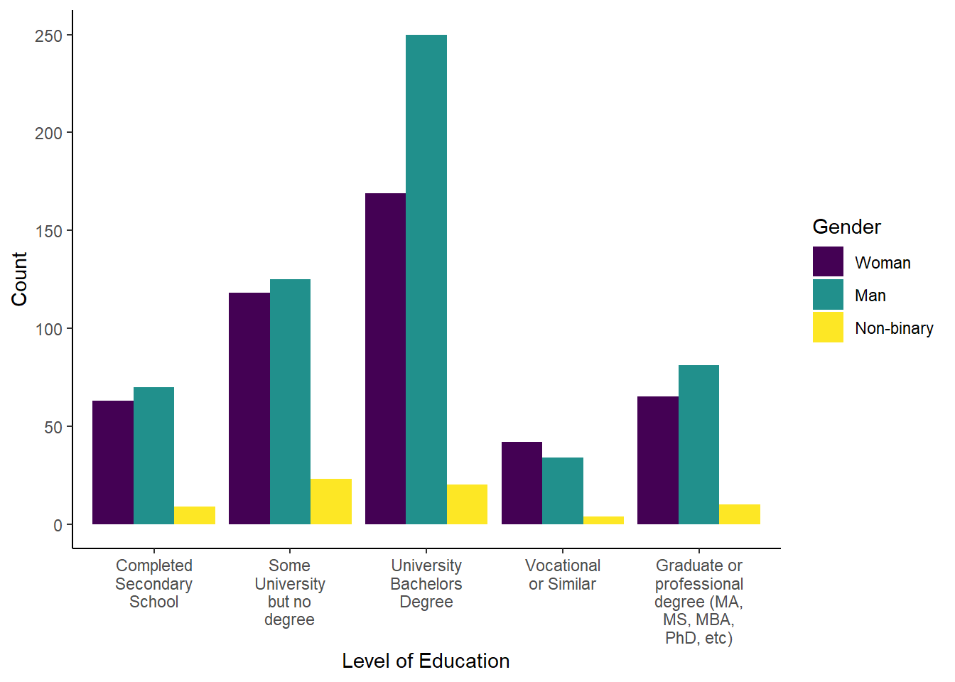
6.5.4 Task 4: Create an appropriate plot
Now we can create the appropriate plot. Which plot would you choose when building one from object chi_square? A with geom layer
Try creating the plot on your own before checking the solution. Feel free to practice adding different layers to make the plot pretty!
6.5.5 Task 5: Compute a chi-square test
Before we can do that, we need to turn our tibble into a dataframe - the associationTest() function we are using to compute the Chi-square test does not like tibbles. [you have nooooo clue how long that took to figure out - let’s say the error message was not exactly helpful]
Now we can run the associationTest() function from the lsr package. The first argument is a formula. It starts with a ~ followed by the two variables you want to associate, separated by a +. The second argument is the dataframe.
Warning in associationTest(formula = ~eduLevel + gender, data = chi_square_df):
Expected frequencies too small: chi-squared approximation may be incorrect
     Chi-square test of categorical association

Variables:   eduLevel, gender

Hypotheses:
   null:        variables are independent of one another
   alternative: some contingency exists between variables

Observed contingency table:
                                                         gender
eduLevel                                                  Woman Man Non-binary
  Completed Secondary School                                 63  70          9
  Some University but no degree                             118 125         23
  University Bachelors Degree                               169 250         20
  Vocational or Similar                                      42  34          4
  Graduate or professional degree (MA, MS, MBA, PhD, etc)    65  81         10

Expected contingency table under the null hypothesis:
                                                         gender
eduLevel                                                  Woman   Man
  Completed Secondary School                               59.9  73.4
  Some University but no degree                           112.2 137.5
  University Bachelors Degree                             185.2 227.0
  Vocational or Similar                                    33.8  41.4
  Graduate or professional degree (MA, MS, MBA, PhD, etc)  65.8  80.7
                                                         gender
eduLevel                                                  Non-binary
  Completed Secondary School                                    8.65
  Some University but no degree                                16.21
  University Bachelors Degree                                  26.75
  Vocational or Similar                                         4.88
  Graduate or professional degree (MA, MS, MBA, PhD, etc)       9.51

Test results:
   X-squared statistic:  13.594
   degrees of freedom:  8
   p-value:  0.093

Other information:
   estimated effect size (Cramer's v):  0.079
   warning: expected frequencies too small, results may be inaccurate
The output is quite informative as it gives information about:
- the variables that were tested,
- the null and alternative hypotheses,
- a table with the observed frequencies (which matches our calculations in
chi_square_frequencywithout the rows/columns of the missing values we removed), - an output of the frequencies you’d expect if the null hypothesis were true,
- the result of the hypothesis test, and
- the effect size Cramer’s v.
It also gives us a warning message saying that expected frequencies are too small and that the chi-squared approximation may be incorrect. This relates to Assumption 4. Depending on your stance on Assumption 4, you may choose to either address or ignore this warning.
The p-value indicates that we do not reject the null hypothesis, as it is greater than 0.05.
6.5.6 Task 6: The write-up
The Chi-Square test revealed that there is no statistically significant association between Gender and Level of Education, \(\chi^2(8) = 13.59, p = .093, V = .079\). The strength of the association between the variables is considered small. We therefore fail to reject the null hypothesis.
6.6 Activity 5: One-sample t-test
The one-sample t-test is used to determine whether a sample comes from a population with a specific mean. This population mean is not always known, but is sometimes hypothesised.
We will perform a one-sample t-test using the continuous variable wemwbs_sum. The official website for the Warwick-Edinburgh Mental Wellbeing Scales states that the “WEMWBS has a mean score of 51.0 in general population samples in the UK with a standard deviation of 7 (Tennant et al., 2007)”.
- Potential research question: “Is the average mental well-being of gamers different from the general population’s average well-being?”
- Null Hypothesis (H0): “The summed-up WEMWBS score of gamers is not different to 51.0.”
- Alternative Hypothesis (H1): “The summed-up WEMWBS score of gamers is different from 51.0.”
6.6.1 Task 1: Preparing the dataframe
First, we need to select the variables of interest: participant ID and wemwbs_sum.
6.6.2 Task 2: Compute descriptives
Next, we want to compute means and standard deviations for our variable of interest. This should be straight forward. Try it yourself and then compare your result with the solution below.
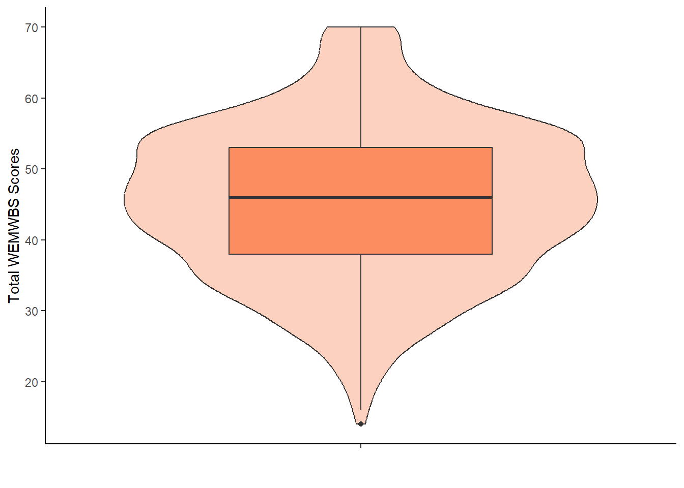
6.6.3 Task 3: Create an appropriate plot
This is the plot you will want to include in your report, so make sure everything is clearly labelled. Which plot would you choose? Try creating one on your own first, then compare it with the solution below.
6.6.4 Task 4: Check assumptions
Assumption 1: Continuous DV
The dependent variable (DV) needs to be measured at interval or ratio level. We can confirm that by looking at one_sample.
Assumption 2: Data are independent
There should be no relationship between the observations. While this is an important assumption, it is more related to study design and isn’t something we can easily test for. Anyway, we will assume this assumption holds for our data.
Assumption 3: No significant outliers
We can check for that visually, for example in the violin-boxplot above.
It appears there is one outlier in the lower tail. However, upon inspecting the one_sample data, we see it is a single participant with a score of 14, which is a possible value. Additionally, with a large sample size of 1,083 participants, removing a single outlier makes not much sense. Thus, we have checked this assumption, considered this outlier not significant, and therefore keep this observation in the dataset.
If you decide to remove any outliers, remember to recalculate the descriptive statistics.
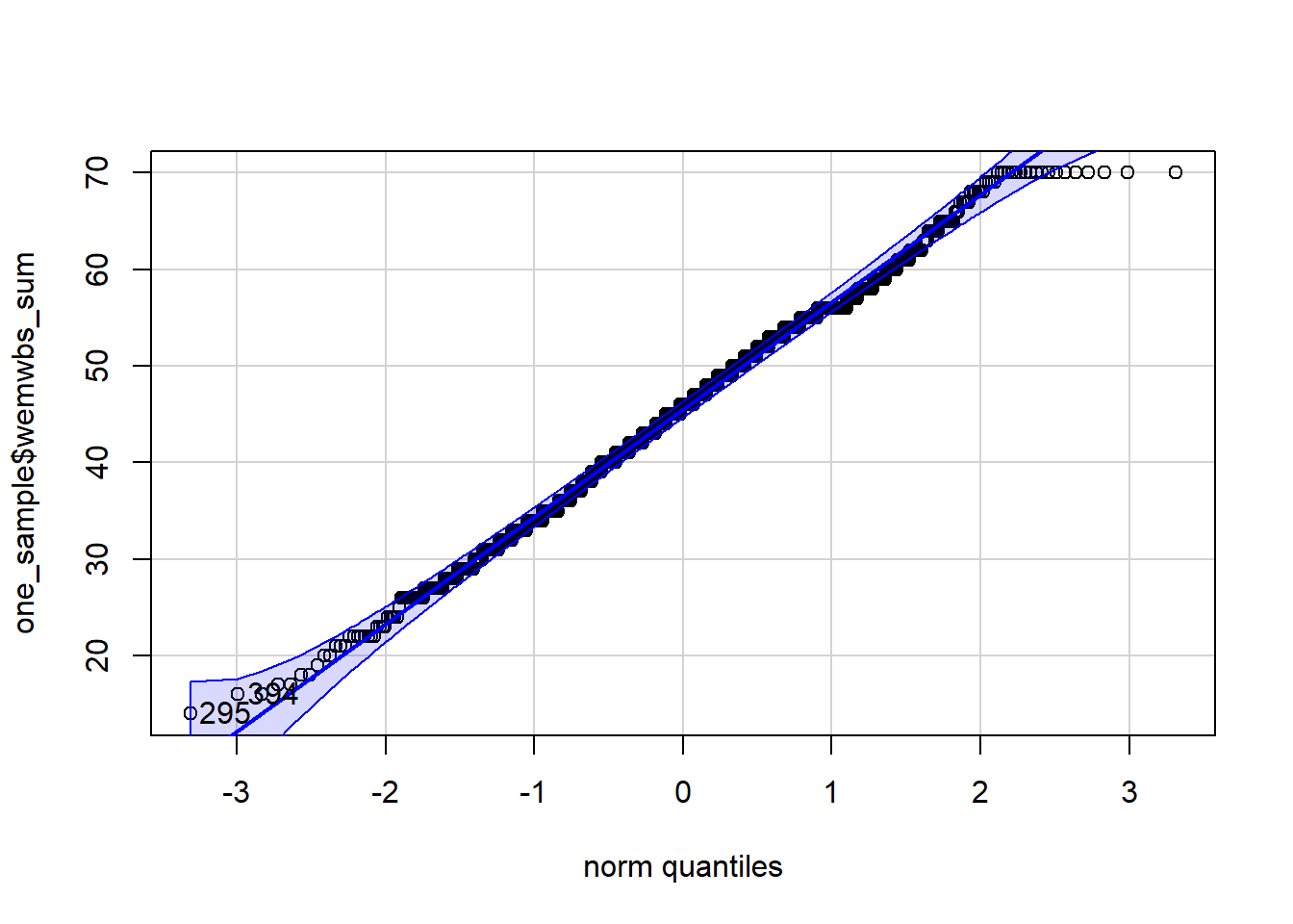
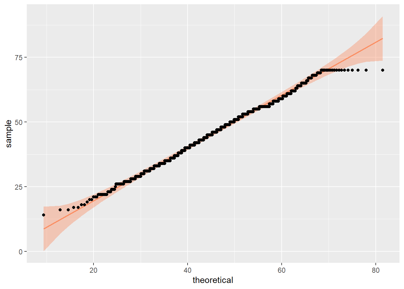
Assumption 4: DV should be approximately normally distributed
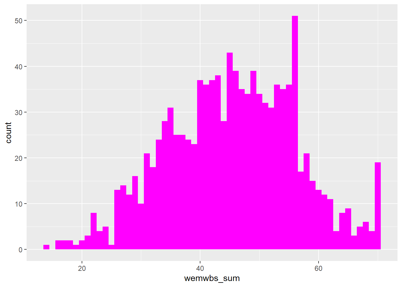
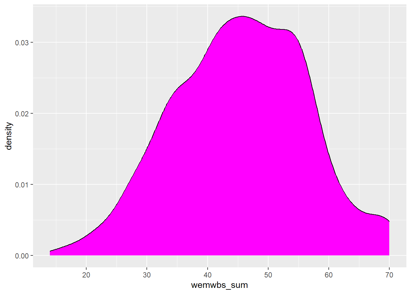
We can already check normality from the violin-boxplot above but you could also use a histogram, a density plot, or a Q-Q plot as an alternative to assess normality visually.
Each of these options shows that the data is normally distributed. This allows us to proceed with a parametric test, specifically a one-sample t-test.
You could also assess normality with the Shapiro-Wilk’s test. The null hypothesis is that the population is distributed normally. Therefore, if the p-value of the Shapiro-Wilk’s test smaller than .05, normality is rejected.
Shapiro-Wilk is an OK method for small sample sizes (e.g., smaller than 50 samples) if the deviation from normality is fairly obvious. If we are dealing with slight deviations from normality, it might not be sensitive enough to pick that up. But t-tests, ANOVAs etc. should be robust for slight deviations from normality anyway.
In contrast, when you have large sample sizes, Shapiro-Wilk is overly sensitive and will definitely produce a significant p-value regardless of what the distribution looks like. So don’t rely on its output when you have large sample sizes, and be mindful of its output when you have small sample sizes.
The function in R for this test is shapiro.test() which is part of BaseR. This means, we need to specify our data object, use the $, and indicate the column we want to address.
    Shapiro-Wilk normality test

data:  one_sample$wemwbs_sum
W = 0.99404, p-value = 0.0002619
No surprise here! The test shows a p-value of < .001 due to our large sample size of over 1000 participants. Nevertheless, if you decided on using the Shapiro-Wilk test in your report, you’d need to write this result up in APA style: \(W = .99, p < .001\).
Either choose visual or computational inspection for normality tests. NO NEED TO DO BOTH!!!
- State what method you used and your reasons for choosing the method (visual/computational and what plot/test you used)
- State the outcome of the test - for visual inspection just say whether normality assumption held or not (no need to include that extra plot in the results section). For computational methods, report the test result in APA style
- State the conclusions you draw from it - parametric or non-parametric test
6.6.5 Task 5: Compute a One-sample t-test and effect size
To compute a one-sample t-test, we can use the t.test() function, which is part of Base R. And yes, you guessed it, our first argument should follow the pattern data$column. The second argument, mu, specifies the population mean we are testing our sample against (in this case, 51.0). The alternative is “two.sided” by default, so it can be omitted if you are conducting a two-sided test.
    One Sample t-test

data:  one_sample$wemwbs_sum
t = -16.868, df = 1082, p-value < 2.2e-16
alternative hypothesis: true mean is not equal to 51
95 percent confidence interval:
 44.77106 46.06920
sample estimates:
mean of x
 45.42013
The output is quite informative. It provides information about:
- the variable column that was tested,
- the t value, degrees of freedom, and p,
- the alternative hypothesis,
- a 95% confidence interval,
- and the mean of the column (which matches the one we computed in the descriptive - yay)
What it doesn’t give us is an effect size. Meh. So we will need to compute one ourselves.
We will calculate Cohen’s d using the function cohensD() from the lsr package. Similar to the t-test we just conducted, the first argument is data$column, the second argument is mu.
6.6.6 Task 6: Sensitivity power analysis
A sensitivity power analysis allows you to determine the minimum effect size that the study could reliably detect given the number of participants you have in the sample (i.e., sample size), the alpha level at 0.05, and an assumed power of 0.8.
To perform this calculation, we use the pwr.t.test() function from the pwr package. This function relies on four key factors — alpha, power, effect size, and sample size (APES). If you know three, you can calculate the fourth. Since we have three specified, we can solve for the effect size. Additionally, we need to specify the type argument to indicate we are using a one-sample t-test, and set alternative to “two.sided” for a non-directional hypothesis.
     One-sample t test power calculation

              n = 1083
              d = 0.08520677
      sig.level = 0.05
          power = 0.8
    alternative = two.sided
So the smallest effect size we can detect with a sample size of 1083, an alpha level of 0.05, and power of 0.8 is 0.09. This is a smaller value than the actual effect size we calculated with our CohensD function above (i.e., 0.51) which means our analysis is sufficiently powered.
6.6.7 Task 7: The write-up
A one-sample t-test was computed to determine whether the average mental well-being of gamers as measured by the WEMWBS was different to the population well-being mean. The average WEMWBS of the gamers \((N = 1083, M = 45.42, SD = 10.89)\) was significantly lower than the population mean well-being score of 51.0, \(t(1082) = 16.87, p < .001, d = .51\). The strength of the effect is considered medium and the study was sufficiently powered. We therefore reject the null hypothesis in favour of H1.
6.7 Activity 6: Non-parametric alternative
If any of the assumptions are violated, switch to the non-parametric alternative. For the one-sample t-test, this would be a One-sample Wilcoxon signed-rank test. Instead of the mean, it compares the median of a sample against a single value (i.e., the population median).
That means we will need to determine the population median, and calculate some summary stats for our sample:
- The population median is listed in a supporting document on the official WEMWBS website as 53.0.
- We can easily calculate the summary statistics using the function
summary().
     pid              wemwbs_sum
 Length:1083        Min.   :14.00
 Class :character   1st Qu.:38.00
 Mode  :character   Median :46.00
                    Mean   :45.42
                    3rd Qu.:53.00
                    Max.   :70.00
The function to compute a one-sample Wilcoxon test is wilcox.test() which is part of BaseR. Code-wise, it works very similar to the one-sample t-test.
    Wilcoxon signed rank test with continuity correction

data:  one_sample$wemwbs_sum
V = 87218, p-value < 2.2e-16
alternative hypothesis: true location is not equal to 53
As we can see, the output shows a V value, but for the final write-up, we need to report the standardised test statistic Z in the final write-up. Unfortunately, this requires manual calculation. According to Andy Field (2012, p. 665), we need to use the qnorm function on the halved p-value from our Wilcoxon test above. Here, we store the p-value in the Global Environment as p_wilcoxon. This retains more decimal places than shown in the output, giving us a more precise Z value.”
# storing the p-value
p_wilcoxon <- wilcox.test(one_sample$wemwbs_sum, mu = 53.0)$p.value

# calculate the z value from half the p-value
z = qnorm(p_wilcoxon/2)
z
[1] -19.12264We also need to calculate the effect size r for the One-sample Wilcoxon signed-rank test. This can be done using the wilcoxonOneSampleR() function from the rcompanion package. By default, the result is rounded to three decimal places, but you can adjust this by adding the digits argument.
Now we have all the numbers we need to write up the results:
A One-sample Wilcoxon signed-rank test was used to compare Gamers’ mental-wellbeing median scores (Mdn = 46.0) to the population median of 53.0. The test showed a significant difference, \(Z = -19.12, p < .001, r = .590\). The strength of the effect is considered medium. We therefore reject the null hypothesis in favour of H1.
Pair-coding
This pair coding task is a bit long to fully complete in class. Try to progress as far as possible without compromising understanding, and treat the remaining section as a “Challenge Yourself” activity.
Intentions behind it?
The task is designed to walk you through conducting a full Chi-Square test on a dataset different from the one in the chapter. I did not want to cherry-pick specific steps from the Chi-Square test, as real-life data analysis requires computing descriptives and checking assumptions before conducting inferential statistics.
Task 1: Open the R project for the lab
Task 2: Create a new .Rmd file
… and name it something useful. If you need help, have a look at Section 1.3.
Task 3: Load in the library and read in the data
The data should already be in your project folder. If you want a fresh copy, you can download the data again here: data_pair_coding.
We are using the packages tidyverse and lsr today, and the data file we need to read in is dog_data_clean_wide.csv. I’ve named my data object dog_data_wide to shorten the name but feel free to use whatever object name sounds intuitive to you.
If you have not worked through chapter 6 yet, you may need to install the package lsr before you can load it into the library. Run install.packages("lsr") in your CONSOLE.
Task 4: Tidy data for a Chi-Square t-test
Look at dog_data_wide and choose two categorical variables. To guide you through this example, I have selected Year of Study and whether or not the students owned pets as my categorical variable.
Step 1: Select all relevant columns from
dog_data_wide. In my case, those would be the participant IDRID,Year_of_Study, andLive_Pets. Store this data in an object calleddog_chi.Step 2: Check if we have any missing values in the
dog_chi. If so remove them with the functiondrop_na().Step 3: Convert
Year_of_StudyandLive_Petsinto factors. Feel free to order the categories meaningfully.
Task 5: Compute descriptives
Create a frequency table (or contingency table to be more exact) from dog_chi, i.e., we need counts for each combination of the variables. Store the data in a new data object dog_chi_contingency. dog_chi_contingency should look like this:
| Year_of_Study | yes | no |
|---|---|---|
| First | 21 | 89 |
| Second | 37 | 64 |
| Third | 12 | 22 |
| Fourth | 12 | 18 |
| Fifth or above | 3 | 2 |
Task 6: Check assumptions
Both variables should be categorical, measured at either the ordinal or nominal level. Answer: as
Year_of_Studyis , andLive_Petsis .Each observation in the dataset has to be independent, meaning the value of one observation does not affect the value of any other. Answer:
Cells in the contingency table are mutually exclusive. Answer: because each individual can belong to in the contingency table.
Task 7: Compute a chi-square test & interpret the output
-
Step 1: Use the function
as.data.frameto turndog_chiinto a dataframe. Store this output in a new data object calleddog_chi_df.
-
Step 2: Run the
associationTest()function from thelsrpackage to compute the Chi-Square test. The structure of the function is as follows:
- Step 3: Interpreting the output
Warning in associationTest(formula = ~Year_of_Study + Live_Pets, data =
dog_chi_df): Expected frequencies too small: chi-squared approximation may be
incorrect
     Chi-square test of categorical association

Variables:   Year_of_Study, Live_Pets

Hypotheses:
   null:        variables are independent of one another
   alternative: some contingency exists between variables

Observed contingency table:
                Live_Pets
Year_of_Study    yes no
  First           21 89
  Second          37 64
  Third           12 22
  Fourth          12 18
  Fifth or above   3  2

Expected contingency table under the null hypothesis:
                Live_Pets
Year_of_Study      yes    no
  First          33.39 76.61
  Second         30.66 70.34
  Third          10.32 23.68
  Fourth          9.11 20.89
  Fifth or above  1.52  3.48

Test results:
   X-squared statistic:  12.276
   degrees of freedom:  4
   p-value:  0.015

Other information:
   estimated effect size (Cramer's v):  0.209
   warning: expected frequencies too small, results may be inaccurate
The Chi-Square test revealed that there is between Year of Study and whether students live with pets, \(\chi^2\) () = , p = , V = . The strength of the association between the variables is considered . We therefore .
Test your knowledge
Question 1: Conceptual Understanding - Chi-Square Test
What is the primary purpose of a Chi-square test?
Question 2: Application - Chi-Square Test
Which of the following scenarios would require a Chi-square test?
Question 3: Interpreting Output - Chi-Square Test
In a Chi-square test, the p-value is .005. What does this imply if the significance level is set at .05?
Question 4: Using R - Chi-Square Test
Which of the following R functions is used to perform a Chi-square test and displays a Cramer’s V in the output?
Question 5: Conceptual Understanding - One-sample t-test
What is the null hypothesis in a one-sample t-test?
Question 6: Application - One-sample t-test
Which of the following scenarios would require a one-sample t-test?
Question 7: Interpreting Output - One-sample t-test
If the p-value in a one-sample t-test is .15 and the significance level is .05, what is the conclusion?
Question 8: Using R - One-sample t-test
Which of the following R functions is used to perform a one-sample t-test?
