8 Paired t-test
Intended Learning Outcomes
By the end of this chapter you should be able to:
- Compute a paired t-test and effectively report the results.
- Understand when to use a non-parametric equivalent of the paired t-test, compute it, and report the results.
Individual Walkthrough
8.1 Activity 1: Setup
In this chapter, we will continue working with the dataset from the study by Zwaan et al. (2018). Have a look at Chapter 7 or the SupMats document if you need a refresher on the Simon Task data.
- Open last week’s project
- Create a new
.Rmdfile and save it to your project folder - Delete everything after the setup code chunk (e.g., line 12 and below)
8.2 Activity 2: Library and data for today
Today, we will need the following packages rstatix, tidyverse, qqplotr, lsr, and pwr. You should have all the necessary packages installed from previous chapters already. If not, you can install them via the console (see Section 1.5.1 for more details).
Again, load the rstatix package before tidyverse. Then read in the data from MeansSimonTask.csv and the demographics information from DemoSimonTask.csv.
As usual, take some time to familiarise yourself with the data before starting the within-subjects t-test.
Today, we will focus on the Simon effect itself. Remember that the Simon effect predicts shorter response times for congruent trials compared to incongruent trials. Therefore, we are inclined to propose a directional hypothesis.
- Potential research question: “Is there a significant difference in response times between congruent and incongruent trials in a Simon task?”
- Null Hypothesis (H0): “There is no significant difference in response times between congruent and incongruent trials in a Simon task.”
- Alternative Hypothesis (H1): “Response times for congruent trials are significantly shorter than those for incongruent trials in a Simon task.” or phrased differently “Participants will respond significantly faster in congruent trials than in incongruent trials in a Simon task.”
8.3 Activity 3: Preparing the dataframe
Again, we need to calculate the mean response time (RT) for both congruent and incongruent trials per participant. As we did last week, we can also compute the Simon effect as the difference score between incongruent and congruent trials.
To keep all the data in one place, we should join this output with the demographics. While you won’t need the demographic information for the t-test itself, having it included will give you a complete dataframe. This can be useful when you need to calculate demographics for the Methods section; for example if you end up excluding data points, you can compute sample size, age, and gender splits straight away rather than having to apply the same exclusion criteria to a different data object.
For the paired version of the t.test, we need the congruent and incongruent trials in separate columns, ensuring each participant still has only one row in the dataframe (i.e., wide format). Below is the output we aim to achieve:
| participant | gender | age | education | similarity | congruent | incongruent | simon_effect |
|---|---|---|---|---|---|---|---|
| T1 | Female | 50 | High school | same | 475.0032 | 508.2835 | 33.28029 |
| T10 | Male | 45 | Associate’s degree | same | 420.1515 | 401.5800 | -18.57148 |
| T109 | Male | 33 | Bachelor’s degree | same | 339.5343 | 375.7152 | 36.18085 |
| T11 | Female | 71 | High school | same | 516.9722 | 542.3111 | 25.33889 |
| T111 | Female | 34 | High school | same | 373.5778 | 394.0665 | 20.48874 |
8.4 Activity 4: Compute descriptives
We want to compute means and standard deviations for both the congruent and the incongruent trials. Then, we will subtract the mean RT of the congruent trials from the mean RT of the incongruent trials to calculate the average difference score between the two conditions.
| mean_congruent | sd_congruent | mean_incongruent | sd_incongruent | diff | sd_diff |
|---|---|---|---|---|---|
| 427.6528 | 74.17418 | 462.0785 | 74.69692 | 34.42571 | 21.59876 |
Notice that we did not have to use group_by() here because the data is already in wide format.
8.5 Activity 5: Create an appropriate plot
8.5.1 Option 1: congruent and incongruent trials
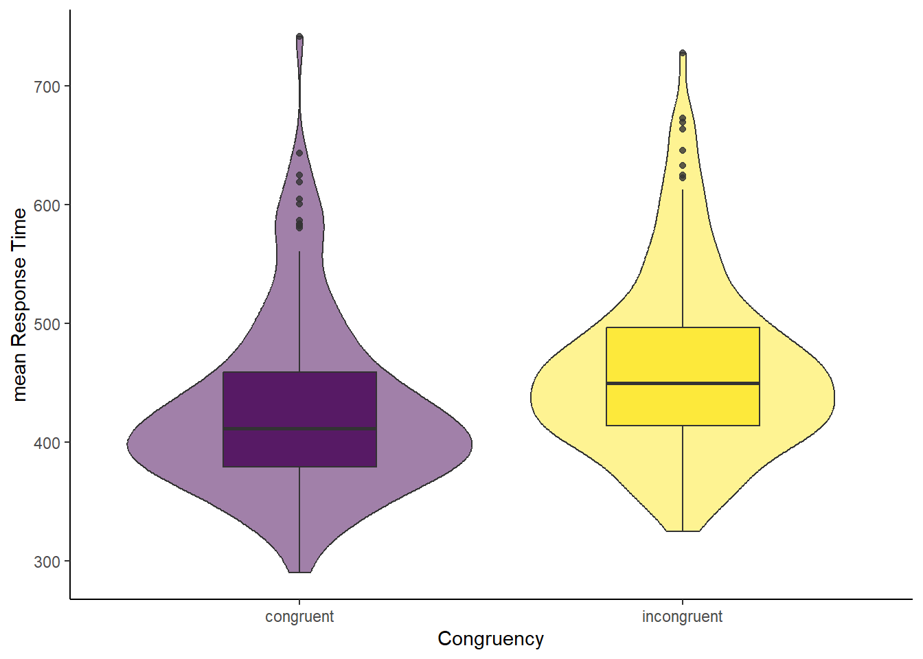
To create an appropriate plot, we need the data in long format. This format should include a congruency column containing the labels for congruent and incongruent trials, and a mean_RT column to store the corresponding mean response times. Each participant should now have two rows in the dataset.
| participant | gender | age | education | similarity | simon_effect | congruency | mean_RT |
|---|---|---|---|---|---|---|---|
| T1 | Female | 50 | High school | same | 33.28029 | congruent | 475.0032 |
| T1 | Female | 50 | High school | same | 33.28029 | incongruent | 508.2835 |
| T10 | Male | 45 | Associate’s degree | same | -18.57148 | congruent | 420.1515 |
| T10 | Male | 45 | Associate’s degree | same | -18.57148 | incongruent | 401.5800 |
| T109 | Male | 33 | Bachelor’s degree | same | 36.18085 | congruent | 339.5343 |
8.5.2 Option 2: difference scores between congruent and incongruent trials
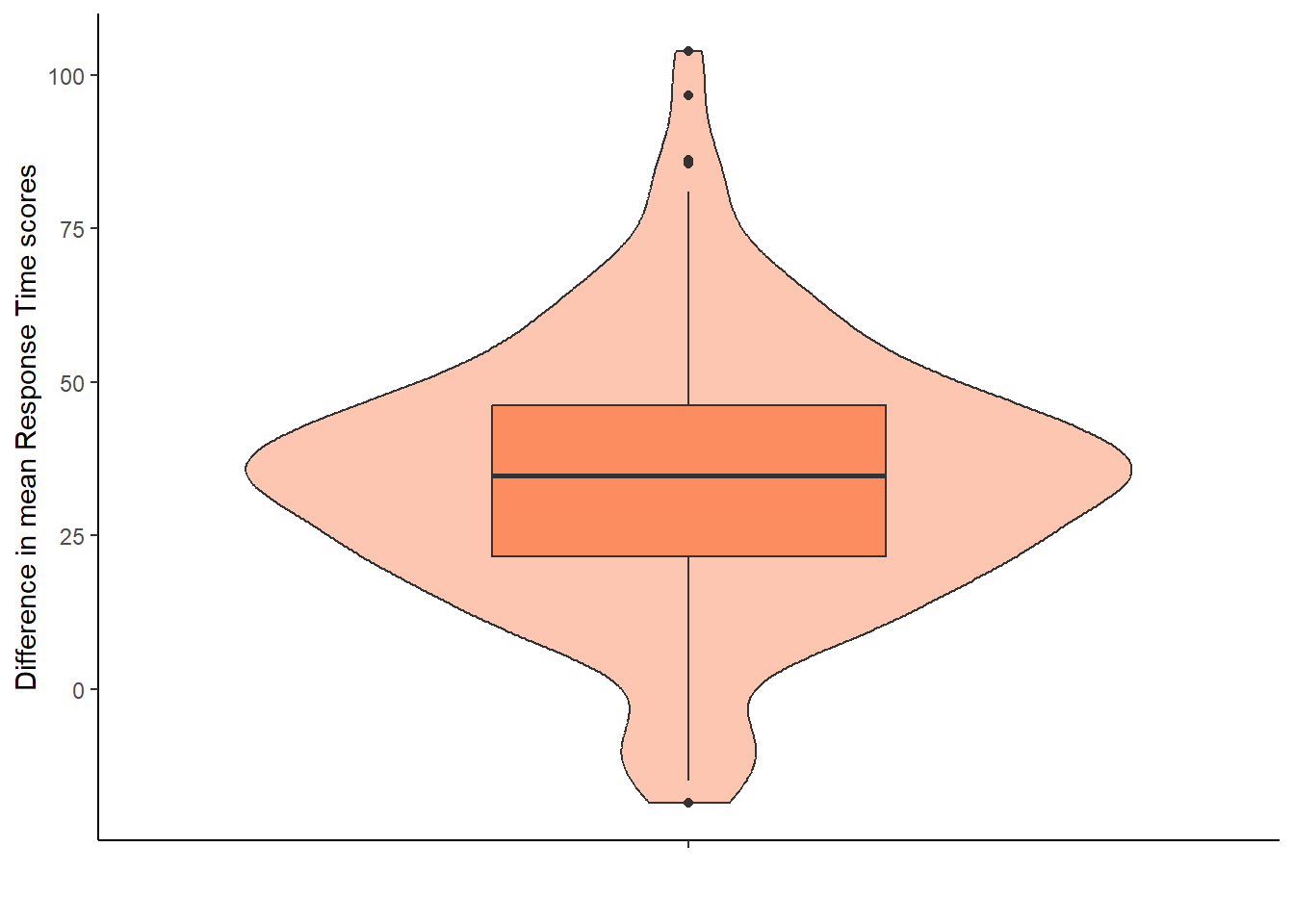
We could have displayed the difference scores between the two conditions directly. This approach would use the simon_effect object without requiring additional data wrangling, as the difference scores are already stored in the simon_effect column.
8.6 Activity 6: Check assumptions
The assumptions for a paired t-test are fairly similar to the one-sample t-test.
Assumption 1: Continuous DV
The dependent variable needs to be measured at interval or ratio level. We can confirm that by looking at either the columns congruent and incongruent in the object simon_effect. Or the variable mean_RT in simon_effect_long. This assumption holds.
Assumption 2: Data are independent
For a paired t-test this assumption applies to the pair of values, i.e., each pair of values needs to be from a separate participant. We assume this assumption holds for our data.
Assumption 3: Normality
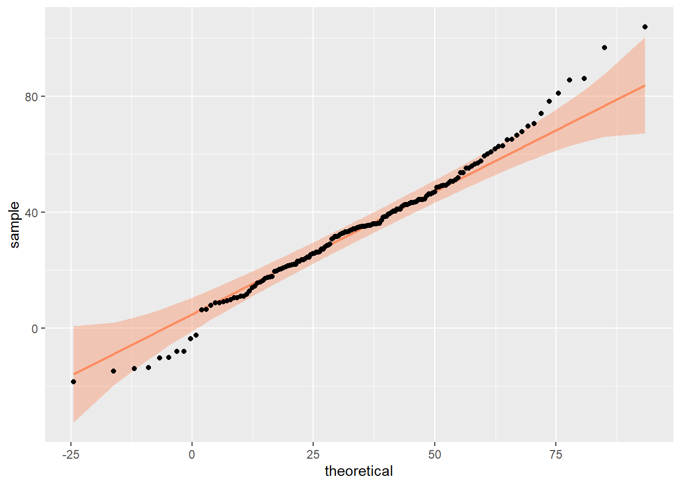
This assumption requires the difference scores to be approximately normally distributed. We cannot see that from the violin-boxplot above (Option 1) and have to plot the difference score, i.e., variable simon_effect.
Assessing normality is never as straightforward as it appears in textbooks. While idealised examples often depict perfectly symmetrical bell curves, real-world data rarely aligns with such precision. Instead, normality exists “on a spectrum”, and it is your responsibility to evaluate whether the data’s shape is sufficiently close to normal for the purposes of your analysis.
This evaluation requires either visual inspection or relying on statistical tests. However, as pointed out in previous chapters, both approaches have limitations and neither provides an absolute answer. Instead of seeking perfection, focus on whether any deviations from normality meaningfully impact the validity of your results.
If any of the assumptions are violated, use the non-parametric equivalent to the paired t-test, see Section 8.10.
8.7 Activity 7: Compute a paired t-test and effect size
We can use the t.test() function again to compute the paired t-test. However, we are stuck with the BaseR pattern data$column once more.
In case you haven’t picked it up by now, I am not much a fan of data$column (i.e., wide format) and prefer the DV ~ IV (i.e., long format) pattern. And there was a time when the t.test() function allowed to add an extra argument paired = TRUE to the formula version but that is no longer the case. 😭😭😭 Now, the argument only works on the default method, specifying arguments x and y separately. And because the default version doesn’t allow us to add a data = argument, we have to revert to data$column.
PS: Carolina disagrees with me and prefers some BaseR every now and then. And that’s totally fine, too - different researchers and coders have their own preferences, which you may have already noticed in the way you code.
Long story short, here are the arguments you need from the data object in wide format (in this case data object simon_effect):
-
data$columnfor condition 1 -
data$columnfor condition 2 - the extra argument
paired = TRUEto tell the function we are conducting a paired rather than a two-sample t-test
    Paired t-test

data:  simon_effect$congruent and simon_effect$incongruent
t = -20.161, df = 159, p-value < 2.2e-16
alternative hypothesis: true mean difference is not equal to 0
95 percent confidence interval:
 -37.79808 -31.05334
sample estimates:
mean difference
      -34.42571
The output tells us pretty much what we need to know:
- the test that was conducted (here a paired t-test),
- the conditions that were compared (here congruent and incongruent),
- the t-value, degrees of freedom, and a p-value,
- the alternative hypothesis,
- a 95% confidence interval,
- and the mean difference score between both conditions (which also matches with our descriptives above).
The t.test() function does not give us an effect size, so, again, we have to compute it ourselves. We can use the CohensD() function from the lsr package as we did for the one-sample and the two-sample t-test. We can use the formula approach here as well, and add the extra argument method = "paired".
The cohensD() function would also take a long format formula approach, such as from simon_effect_long, but you would need to make sure that the data within the columns are ordered correctly, i.e., Participant 1: condition 1, condition 2; Participant 2: condition 1, condition 2; etc. If that’s not the case, then your results will be wrong. R helpfully provides a warning message for you to notice and double-check your data accordingly.
Warning in cohensD(mean_RT ~ congruency, data = simon_effect_long, method =
"paired"): calculating paired samples Cohen's d using formula input. Results
will be incorrect if cases do not appear in the same order for both levels of
the grouping factor
[1] 1.5938748.8 Activity 8: Sensitivity power analysis
As with the other t-test, we are conducting a sensitivity power analysis to determine the minimum effect size detectable with the number of participants we have in our sample (here n = 160), alpha of 0.05 and power of 0.8. This will tell us if our analysis was sufficiently powered or not.
The function we will use again is pwr.t.test() from the pwr package. The arguments in the formula are the same as for the one-sample t-test; we just need to adjust the number of participants and set the type to “paired”.
     Paired t test power calculation

              n = 160
              d = 0.222858
      sig.level = 0.05
          power = 0.8
    alternative = two.sided

NOTE: n is number of *pairs*
The minimum effect size we could reliably detect is 0.22. Our actual effect size was 1.59, so this analysis was sufficiently powered. YAY
8.9 Activity 9: The write-up
We hypothesised that there would be a significant difference in the response times between congruent \((M = 427.65 msec, SD = 74.17 msec)\) and incongruent trials \((M = 462.08 msec, SD = 74.70 msec)\) of a Simon task. On average, participants were faster in the congruent compared to the incongruent condition \((M_{diff} = 34.43 msec, SD_{diff} = 21.60 msec)\). Using a within-subjects t-test, the effect was found to be significant and of a large magnitude, \(t(159) = 20.16, p < .001, d = 1.59\). Therefore, we reject the null hypothesis in favour of H1.
8.10 Activity 10: Non-parametric alternative
The Wilcoxon signed-rank test is the non-parametric equivalent to the paired t-test, comparing the difference between the median for two measurements.
Before we compute the test, we need to determine some summary stats (e.g., here we focus on the median scores) for the congruent and incongruent conditions. Similar to the One-sample Wilcoxon signed-rank test, we can use the summary() function again because our data is in wide format.
 participant           gender               age         education
 Length:160         Length:160         Min.   :19.00   Length:160
 Class :character   Class :character   1st Qu.:30.75   Class :character
 Mode  :character   Mode  :character   Median :37.00   Mode  :character
                                       Mean   :39.86
                                       3rd Qu.:49.00
                                       Max.   :71.00
  similarity          congruent      incongruent     simon_effect
 Length:160         Min.   :290.0   Min.   :324.9   Min.   :-18.57
 Class :character   1st Qu.:379.4   1st Qu.:413.9   1st Qu.: 21.62
 Mode  :character   Median :411.3   Median :449.7   Median : 34.77
                    Mean   :427.7   Mean   :462.1   Mean   : 34.43
                    3rd Qu.:458.7   3rd Qu.:496.3   3rd Qu.: 46.22
                    Max.   :741.5   Max.   :727.9   Max.   :103.84
Now we can move on to the Wilcoxon signed-rank test. We will use the wilcox.test() function again, but add the argument paired = TRUE.
    Wilcoxon signed rank test with continuity correction

data:  simon_effect$congruent and simon_effect$incongruent
V = 144, p-value < 2.2e-16
alternative hypothesis: true location shift is not equal to 0We could have also run a One-sample Wilcoxon signed-rank test on the difference score, but instead of comparing that to a population median (as we did in Section 6.7), we would compare it to 0 to assess whether the median difference between paired observations is significantly different from zero.
    Wilcoxon signed rank test with continuity correction

data:  simon_effect$simon_effect
V = 12736, p-value < 2.2e-16
alternative hypothesis: true location is not equal to 0Yes and no. The order in which you input variables into the function will affect the value of V - has to do with how the ranks are getting assigned. In our column simon_effect we subtracted congruent RT from incongruent RT. To have the exact equivalent, we will need to switch the columns in the wilcox.test() function.
    Wilcoxon signed rank test with continuity correction

data:  simon_effect$incongruent and simon_effect$congruent
V = 12736, p-value < 2.2e-16
alternative hypothesis: true location shift is not equal to 0
And as you can see, the V values match now.
We should also compute the standardised test statistic Z. Again, we need to calculate Z manually, using the qnorm function on the halved p-value from our Wilcoxon test above.
# storing the p-value
p_wilcoxon <- wilcox.test(simon_effect$incongruent, simon_effect$congruent, paired = TRUE)$p.value

# calculate the z value from half the p-value
z = qnorm(p_wilcoxon/2)
z
[1] -10.72532To calculate an effect size, we would need to use the function wilcox_effsize() from the rstatix package. Unlike, the wilcox.test() and the t.test() function, wilcox_effsize() expects data to be in long format to be able to use the DV ~ IV pattern. Fortunately, we still have that available in simon_effect_long. We also need to add the argument paired = TRUE.
| .y. | group1 | group2 | effsize | n1 | n2 | magnitude |
|---|---|---|---|---|---|---|
| mean_RT | congruent | incongruent | 0.8479786 | 160 | 160 | large |
Now we have all the numbers to write this up:
A Wilcoxon signed-rank test was conducted to determine whether there was a significant difference in response times between congruent \((Mdn = 411.3 msec)\) and incongruent trials \((Mdn = 449.7 msec)\) in a Simon task. Median response times of Congruent trials were significantly faster \((Mdn = 34.77 msec)\) than incongruent trials, \(Z = -10.73, p < .001, r = .848\). The difference can be classified as large according to Cohen (1992). Therefore, we reject the null hypothesis in favour of H1.
Pair-coding
This week’s pair-coding activity mirrors the one from Chapter 7. While there is no lab scheduled this week, I wanted to provide an opportunity for you to practice. You can treat this either as a “Challenge Yourself” activity or get together with friends to work through it together.
Task 1: Open the R project for the lab
Task 2: Create a new .Rmd file
… and name it something useful. If you need help, have a look at Section 1.3.
Task 3: Load in the library and read in the data
The data should already be in your project folder. If you want a fresh copy, you can download the data again here: data_pair_coding.
We are using the packages rstatix, tidyverse, qqplotr, lsr today. Make sure to load rstatix in before tidyverse.
We also need to read in dog_data_clean_wide.csv. Again, I’ve named my data object dog_data_wide to shorten the name but feel free to use whatever object name sounds intuitive to you.
For the plot, we will need the data in long format. We can either read in dog_data_clean_long.csv to take a shortcut, or wrangle the data from dog_data_wide. I’ve taken the shortcut and named my data object dog_data_long.
Task 4: Tidy data for a paired t-test
Not much tidying to do for today.
Pick a variable of interest and select the pre- and post-scores, and calculate the difference score. Store them in a separate data object with a meaningful name.
I will use Loneliness as an example and call my data object dog_lonely. Regardless of your chosen variable, your data object should look like/ similar to the table below.
| RID | Loneliness_pre | Loneliness_post | Loneliness_diff |
|---|---|---|---|
| 1 | 2.25 | 1.70 | -0.55 |
| 2 | 1.90 | 1.60 | -0.30 |
| 3 | 2.25 | 2.25 | 0.00 |
| 4 | 1.75 | 2.05 | 0.30 |
| 5 | 2.85 | 2.70 | -0.15 |
In dog_data_long, we want to turn Stage into a factor so we can re-order the labels (i.e., “pre” before “post”).
Task 5: Compute descriptives
We want to determine the mean and sd of:
- the pre-scores
- the post-scores, and
- the difference scores
Store them in a data object called descriptives.
Task 6: Check assumptions
Assumption 1: Continuous DV
Is the dependent variable (DV) continuous? Answer:Assumption 2: Data are independent
Each pair of values in the dataset has to be independent, meaning each pair of values needs to be from a separate participant. Answer:
Assumption 3: Normality
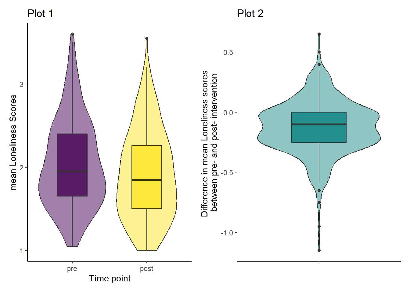
Looking at the violin-boxplots below, do you think the assumption of normality holds?
The labels of Plot 2 turned out to be quite long here. I’ve used the escape character \n here. to break up the title across 2 lines.
## Plot 1
ggplot(dog_data_long, aes(x = Stage, y = Loneliness, fill = Stage)) +
  geom_violin(alpha = 0.5) +
  geom_boxplot(width = 0.4, alpha = 0.8) +
  scale_fill_viridis_d(guide = "none") +
  theme_classic() +
  labs(x = "Time point", y = "mean Loneliness Scores")

## Plot 2
ggplot(dog_lonely, aes(x = "", y = Loneliness_diff)) +
  geom_violin(fill = "#21908C", alpha = 0.5) +
  geom_boxplot(fill = "#21908C", width = 0.4) +
  theme_classic() +
  labs(x = "",
       y = "Difference in mean Loneliness scores \nbetween pre- and post- intervention") # \n forces a manual line break in the axis label
Answer:
Conclusion from assumption tests
With all assumptions tested, which statistical test would you recommend for this analysis?
Answer:Task 7: Computing a paired-sample t-test with effect size & interpret the output
- Step 1: Compute the paired-sample t-test. The structure of the function is as follows:
- Step 2: Calculate an effect size
Calculate Cohen’s D. The structure of the function is as follows:
- Step 3: Interpreting the output
Below are the outputs for the descriptive statistics (table), paired-samples t-test (main output), and Cohen’s D (last line starting with [1]). Based on these, write up the results in APA style and provide an interpretation.
| mean_pre | sd_pre | mean_post | sd_post | diff | sd_diff |
|---|---|---|---|---|---|
| 2.040187 | 0.5304488 | 1.914298 | 0.5344914 | -0.1258895 | 0.2290269 |
    Paired t-test

data:  dog_lonely$Loneliness_pre and dog_lonely$Loneliness_post
t = 9.2632, df = 283, p-value < 2.2e-16
alternative hypothesis: true mean difference is not equal to 0
95 percent confidence interval:
 0.09913876 0.15264034
sample estimates:
mean difference
      0.1258895

[1] 0.5496716
We hypothesised that there would be a significant difference between Loneliness measured before (M = , SD = ) and after (M = , SD = ) the dog intervention. On average, participants felt less lonely after the intervention (Mdiff = , SDdiff = ). Using a paired-samples t-test, the effect was found to be and of a magnitude, t() = , p , d = . We therefore .
Test your knowledge
Question 1
What is the main purpose of an paired-samples t-test?
Question 2
Which of the following is a key assumption of the paired t-test?
Question 3
What is the null hypothesis for a paired t-test?
Question 4
A paired-samples t-test was conducted to compare sleep quality scores with (M = 7.5, SD = 1.8) and without (M = 6.0, SD = 1.9) white noise, t(29) = 4.55, p < .001, d = 0.82. Answer the questions below.
- How many participants were included in the study?
- What is the effect size, and how would you describe its magnitude? The effect size is and of magnitude.
- Is the result statistically significant?
- Based on the means and standard deviations, how would you summarise the direction of the effect?


