13 Factorial ANOVA

Intended Learning Outcomes

By the end of this chapter you should be able to:

Apply and interpret a factorial ANOVA.
Break down the results of a factorial ANOVA using post hoc tests and apply a correction for multiple comparisons.
Check statistical assumptions for factorial ANOVA through your understanding of the design and diagnostic plots.
Visualise the results of a factorial ANOVA through an interaction plot.

Individual Walkthrough

13.1 Activity 1: Setup & download the data

This week, we will be working with a new dataset - Experiment 3 in Zhang et al. (2014). Follow the steps below to set up your project:

Create a new project and name it something meaningful (e.g., “2B_chapter13”, or “13_anova”). See Section 1.2 if you need some guidance.
Create a new .Rmd file and save it to your project folder. See Section 1.3 if you need help.
Delete everything after the setup code chunk (e.g., line 12 and below)
Download the new dataset here: data_ch13.zip. The zip folder includes:
- the data file for Study 3 (Zhang_2014_Study3.csv)
- the codebook for Study (Zhang_2014_Study3_codebook.xlsx), and the
- a document explaining the Materials and Methods of Study 3 (Materials_and_methods_Study3.docx).
Extract the data file from the zip folder and place it in your project folder. If you need help, see Section 1.4.

Citation

Zhang, T., Kim, T., Brooks, A. W., Gino, F., & Norton, M. I. (2014). A “Present” for the Future: The Unexpected Value of Rediscovery. Psychological Science, 25(10), 1851-1860. https://doi.org/10.1177/0956797614542274

Abstract

Although documenting everyday activities may seem trivial, four studies reveal that creating records of the present generates unexpected benefits by allowing future rediscoveries. In Study 1, we used a time-capsule paradigm to show that individuals underestimate the extent to which rediscovering experiences from the past will be curiosity provoking and interesting in the future. In Studies 2 and 3, we found that people are particularly likely to underestimate the pleasure of rediscovering ordinary, mundane experiences, as opposed to extraordinary experiences. Finally, Study 4 demonstrates that underestimating the pleasure of rediscovery leads to time-inconsistent choices: Individuals forgo opportunities to document the present but then prefer rediscovering those moments in the future to engaging in an alternative fun activity. Underestimating the value of rediscovery is linked to people’s erroneous faith in their memory of everyday events. By documenting the present, people provide themselves with the opportunity to rediscover mundane moments that may otherwise have been forgotten.

The data is available on OSF: https://osf.io/t2wby/

In summary, the researchers were interested in whether people could accurately predict how interested they would be in revisiting past experiences. They referred to this as the “time capsule” effect, where individuals store photos or messages to remind themselves of past events in the future. The researchers predicted that participants in the ordinary condition would underestimate their future feelings (i.e., show a greater difference between time 1 and time 2 ratings) compared to those in the extraordinary condition.

Changes made to the dataset

The original SPSS file was converted to CSV format. Columns are already tidied.
No other changes were made.

13.2 Activity 2: Load in the library, read in the data, and familiarise yourself with the data

Today, we will use several packages: afex, tidyverse, performance, emmeans, and effectsize.

We also need to read in the dataset Zhang_2014_Study3.csv

???

data_zhang <- ???

Solution

library(afex)
library(tidyverse)
library(performance)
library(emmeans)
library(effectsize)

data_zhang <- read_csv("Zhang_2014_Study3.csv")

13.3 Activity 3: Preparing the dataframe

This is a 2 x 2 mixed factorial ANOVA, with one within-subjects factor (time: time 1 vs. time 2) and one between-subjects factor (type of event: ordinary vs. extraordinary).

So let’s start by wrangling the data we need for today’s analysis:

Only include participants who completed the questionnaire at both time point 1 and time point 2.
Add a column called Participant_ID. We did that last week.
Convert the column Condition into a factor.
Select the following columns
- Participant_ID
- Gender
- Age
- Condition
- The predicted interest composite score at time point 1 T1_Pred_Interest_Comp and relabel it as Time 1
- The actual interest composite score at time point 2 T2_Interest_Comp and relabel it as Time 2
Store the cleaned dataset as zhang_data.

We should also create a long format version zhang_long that stores the interest composite scores for time points 1 and 2 in a single column (see excerpt below). Obviously zhang_long should have data from all 130 participants, not just the first 3.

Participant_ID	Gender	Age	Condition	Time_Point	Interest_Composite_Score
1	Female	22	Ordinary	Time 1	3.25
1	Female	22	Ordinary	Time 2	4.50
2	Male	23	Ordinary	Time 1	2.00
2	Male	23	Ordinary	Time 2	1.50
3	Female	26	Ordinary	Time 1	5.00
3	Female	26	Ordinary	Time 2	6.50

Solution

zhang_data <- data_zhang %>% 
  filter(T2_Finished == "Yes") %>% 
  mutate(Participant_ID = row_number(),
         Condition = factor(Condition)) %>% 
  select(Participant_ID, Gender, Age, Condition, `Time 1` = T1_Pred_Interest_Comp, `Time 2` = T2_Interest_Comp)

zhang_long <- zhang_data %>% 
  pivot_longer(cols = `Time 1`:`Time 2`,
               names_to = "Time_Point",
               values_to = "Interest_Composite_Score")

13.4 Activity 4: Compute descriptives

Now, we can calculate the number of participants in each group, as well as means, and standard deviations for each level of IV, and for both IVs overall.

Bonus: round the numbers to 2 decimal places

Hints

You cannot do this all in one go. One option is to compute all required variables for Time, Condition, and grouped by Time and Condition separately, and then combine all dataframes.
The final output should contain 8 observations and 5 variables.
To round the values, use the round() function by wrapping it around the mean() and sd() functions.

Solution

## grouped output
descriptives <- zhang_long %>%
  group_by(Condition, Time_Point) %>%
  summarise(n = n(),
            mean = round(mean(Interest_Composite_Score), 2), 
            sd = round(sd(Interest_Composite_Score), 2)) %>% 
  ungroup()

`summarise()` has grouped output by 'Condition'. You can override using the
`.groups` argument.

descriptives_T <- zhang_long %>%
  group_by(Time_Point) %>%
  summarise(n = n(),
            mean = round(mean(Interest_Composite_Score), 2), 
            sd = round(sd(Interest_Composite_Score), 2)) %>% 
  ungroup() %>% 
  mutate(Condition = "all")

descriptives_C <- zhang_long %>%
  group_by(Condition) %>%
  summarise(n = n(),
            mean = round(mean(Interest_Composite_Score), 2), 
            sd = round(sd(Interest_Composite_Score), 2)) %>% 
  ungroup() %>% 
  mutate(Time_Point = "all")

descriptives <- descriptives %>% 
  full_join(descriptives_T) %>% 
  full_join(descriptives_C)

Joining with `by = join_by(Condition, Time_Point, n, mean, sd)`
Joining with `by = join_by(Condition, Time_Point, n, mean, sd)`

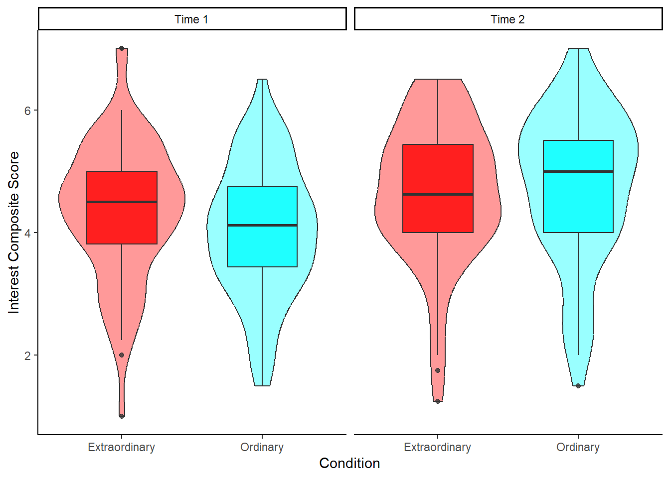
13.5 Activity 5: Create an appropriate plot

Try to recreate the following violin-boxplot. See how many features you can replicate before checking the code. The colour palette might be a bit tricky, but the rest should be fairly straightforward.

Hint for the colour palette

The colour palette used here is one we haven’t explored yet. It’s called rainbow() and is a built-in palette in BaseR. To apply it, you can define it as the values argument within the scale_fill_manual() function.

Solution

ggplot(zhang_long, aes(x = Condition, y = Interest_Composite_Score, fill = Condition)) +
  geom_violin(alpha = 0.4) + 
  geom_boxplot(width = 0.5, alpha = 0.8) +
  facet_wrap(~ Time_Point) +
  theme_classic() +
  scale_fill_manual(values=rainbow(2),
                    guide = "none") +
  labs(y = "Interest Composite Score")

13.6 Activity 6: Store the ANOVA model and check assumptions

13.6.1 The ANOVA model

This week, we will use the aov_ez() function from the afex package to run our analysis and save the model. The arguments are very similar to the anova_test() function we used last week, so the switch should feel familiar. However, while anova_test() does run the anova, somehow it doesn’t store the full model object properly when defining the arguments manually. As that makes it difficult to run post-hoc tests or check assumptions, we are switching to aov_ez() to give ourselves more flexibility for assumption checks and follow-up analyses.

The aov_ez() function requires the following arguments:

aov_ez(id = "NULL",
       data = NULL, 
       between = "NULL", 
       within = "NULL",
       dv = "NULL", 
       type = 3,
       anova_table = list(es = "NULL"))

id = The column name of the participant identifier (factor).
data = The data object.
between = The between-subjects factor variable(s).
within = The within-subjects factor variable(s).
dv = The dependent variable (DV; numeric).
type = The type of sums of squares for ANOVA (here we need Type 3).
anova_table = list(es = "NULL") specifies the effect size to compute (here we set “NULL” to “pes” for partial eta squared).

Now define the parameters for your analysis based on our current dataset. Check the solution when you’re done. Store the model in an object called mod.

Solution

mod <- aov_ez(id = "Participant_ID",
       data = zhang_long, 
       between = "Condition", 
       within = "Time_Point",
       dv = "Interest_Composite_Score", 
       type = 3,
       anova_table = list(es = "pes"))

Contrasts set to contr.sum for the following variables: Condition

13.6.2 Assumption checks

The assumptions for a factorial ANOVA are the same as the one-way ANOVA.

Assumption 1: Continuous DV

The dependent variable (DV) must be measured at the interval or ratio level. In our case, this assumption is met.

Deep Dive: Ordinal data

Ordinal data are commonly found in psychology, especially in the form of Likert scales. The challenge is that ordinal data are not interval or ratio data. They consist of a fixed set of ordered categories (e.g., the points on a Likert scale), but we can’t assume the distances between those points are equal. For example, is the difference between strongly agree and agree really the same as the difference between agree and neutral?

Technically, we shouldn’t use ANOVA to analyse ordinal data. But in practice, almost everyone does. A common justification is that when you average multiple Likert-scale items, the resulting composite score can be treated as interval data and may approximate a normal distribution.

Others argue that non-parametric tests or more advanced models like ordinal regression are more appropriate for ordinal data. However, this is beyond the scope of what we cover in this course.

Whichever approach you choose, the key is to understand the data you have and be able to justify your analytical decision.

Assumption 2: Data are independent

This assumption holds due to the study design; each participant provided responses independently.

Assumption 3: Normality

The residuals of the DV should be normally distributed.

This assumption can be checked using the check_model() function from the performance package.

check_model(mod)

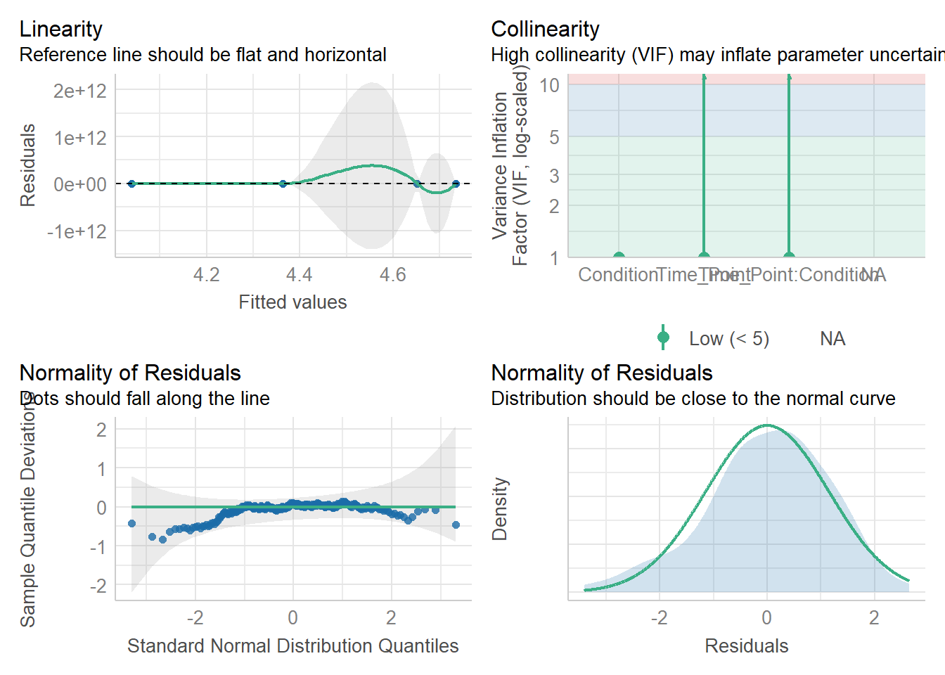
As we can see here, the assumption is met. The residuals are approximately normally distributed. In both normality plots displayed, you can see they fall close to the horizontal reference line, and the density plot shows a roughly bell-shaped distribution.

Assumption 4: Homoscedasticity

The variances across groups should be approximately equal.

We can test this using the check_homogeneity() function from the performance package. Simply run it on your model object mod. This function uses Levene’s Test to assess whether the variances across all four groups (i.e., the cells of our 2 × 2 design) are roughly equal:

check_homogeneity(mod, method = "levene")

OK: There is not clear evidence for different variances across groups (Levene's Test, p = 0.893).

You can also visualise the results:

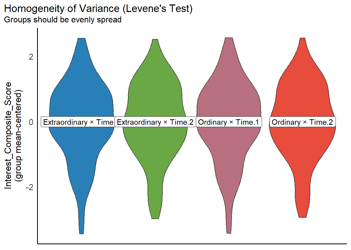
plot(check_homogeneity(mod, method = "levene"))

In this case, the non-significant p-value suggests that the variances across the four groups are roughly equal. The assumption is therefore met. This is also evident from the plot, which shows relatively similar spread across groups.

13.7 Activity 7: Compute a mixed factorial ANOVA

Since we already stored the model above, all that’s left is to run the output. To view the ANOVA results, simply call the model object:

mod

Anova Table (Type 3 tests)

Response: Interest_Composite_Score
                Effect     df  MSE         F  pes p.value
1            Condition 1, 128 2.05      0.46 .004    .498
2           Time_Point 1, 128 0.61 25.88 *** .168   <.001
3 Condition:Time_Point 1, 128 0.61    4.44 * .034    .037
---
Signif. codes:  0 '***' 0.001 '**' 0.01 '*' 0.05 '+' 0.1 ' ' 1

Look at the results, and answer the following questions:

Is the main effect of Condition significant?
Is the main effect of Time significant?
Is the two-way interaction significant?

13.8 Activity 8: Compute post-hoc tests, an interaction plot, and effect sizes

13.8.1 Post-hoc comparisons

13.8.1.1 Main effect of Time Point

We do not need to run emmeans() for a post hoc comparison, because Time_Point only has 2 levels.

However, seeing that Zhang et al. report Confidence Intervals in their final write-up and we didn’t calculate them earlier, we could use emmeans() to achieve that quickly.

emmeans(mod, ~ Time_Point)

 Time_Point emmean     SE  df lower.CL upper.CL
 Time.1       4.20 0.0977 128     4.01     4.39
 Time.2       4.69 0.1044 128     4.49     4.90

Results are averaged over the levels of: Condition 
Confidence level used: 0.95

13.8.1.2 Interaction of Time Point and Condition

Because the interaction is significant, we should follow up with post hoc tests using the emmeans() function to determine which specific group comparisons are driving the effect. If the interaction is not significant, there is no justification for conducting these post hoc tests.

The emmeans() function requires you to specify the model object, and then the factors you want to contrast, here our interaction term (Time_Point*Condition).

emmeans(mod, ~ Time_Point*Condition)

 Time_Point Condition     emmean    SE  df lower.CL upper.CL
 Time.1     Extraordinary   4.36 0.137 128     4.09     4.63
 Time.2     Extraordinary   4.65 0.147 128     4.36     4.94
 Time.1     Ordinary        4.04 0.139 128     3.76     4.31
 Time.2     Ordinary        4.73 0.149 128     4.44     5.03

Confidence level used: 0.95

This gives us the estimated marginal means for each combination of the two independent variables. As you can see, these values match the descriptives we computed earlier. However, we still need to compute the contrasts to determine which comparisons are statistically significant.

We can use the contrast() function, piped onto the output of emmeans() do get the constrast comparisons. Here’s how it works:

interaction = "pairwise" specifies that we want to test pairwise contrasts within the interaction, i.e., comparisons at each level of the other variable.
simple = "each" tells R to test each factor separately across the levels of the other factor. If we leave this out, it will test the difference between time points and event types as a single contrast, which isn’t meaningful in this context.
combine = FALSE ensures that p-value adjustments are applied separately at each level of the other variable. If set to TRUE, all comparisons would be pooled and corrected together. You might choose combine = FALSE when you’re interested in simple effects (e.g., differences within each condition separately), and combine = TRUE when you’re making a larger number of comparisons across the full interaction and want a more conservative correction.
adjust = "bonferroni" specifies the method for correcting multiple comparisons. However, in a 2 × 2 design, if combine = FALSE, there is only one comparison per level of the other factor. So no correction is actually applied, as there’s nothing to adjust for.

emmeans(mod, ~ Time_Point*Condition) %>% 
  contrast(interaction = "pairwise", 
           simple = "each", 
           combine = FALSE, 
           adjust = "bonferroni")

$`simple contrasts for Time_Point`
Condition = Extraordinary:
 Time_Point_pairwise estimate    SE  df t.ratio p.value
 Time.1 - Time.2       -0.288 0.136 128  -2.123  0.0357

Condition = Ordinary:
 Time_Point_pairwise estimate    SE  df t.ratio p.value
 Time.1 - Time.2       -0.695 0.138 128  -5.049  <.0001


$`simple contrasts for Condition`
Time_Point = Time.1:
 Condition_pairwise       estimate    SE  df t.ratio p.value
 Extraordinary - Ordinary   0.3246 0.195 128   1.661  0.0992

Time_Point = Time.2:
 Condition_pairwise       estimate    SE  df t.ratio p.value
 Extraordinary - Ordinary  -0.0829 0.209 128  -0.397  0.6923

13.8.2 Creating an interaction plot

When you have a factorial design, one powerful way of visualising the data is through an interaction plot. This is essentially a line graph where the x-axis has one IV and separate lines for a second IV. However, once you have the factorial ANOVA model, you can add confidence intervals to the plot to visualise uncertainty. The afex package has its own function called afex_plot() which you can use with the model object you created.

In the code below, there are a few key argument to highlight:

object is the model you created.
x is the variable you want on the x-axis.
trace is the variable you want to plot as separate lines.
error controls whether the error bars show confidence intervals for between-subjects or within-subjects. In a mixed design, these have different properties, so you must think about which you want to plot and highlight to the reader.
factor_levels lets you edit the levels of factors you plot, such as renaming or reordering them.

Plus, afex_plot() uses ggplot2 in the background, so you can add layers to the initial function land use ggsave() if you wanted to save your plot

afex_plot(object = mod, 
          x = "Condition", 
          trace = "Time_Point", 
          error = "between",
          factor_levels = list(Time_Point = c("Time 1", "Time 2"))) + 
  theme_classic() + 
  scale_y_continuous(breaks = 1:7)

Renaming/reordering factor levels of 'Time_Point':
  Time.1 -> Time 1
  Time.2 -> Time 2

Warning: Panel(s) show a mixed within-between-design.
Error bars do not allow comparisons across all means.
Suppress error bars with: error = "none"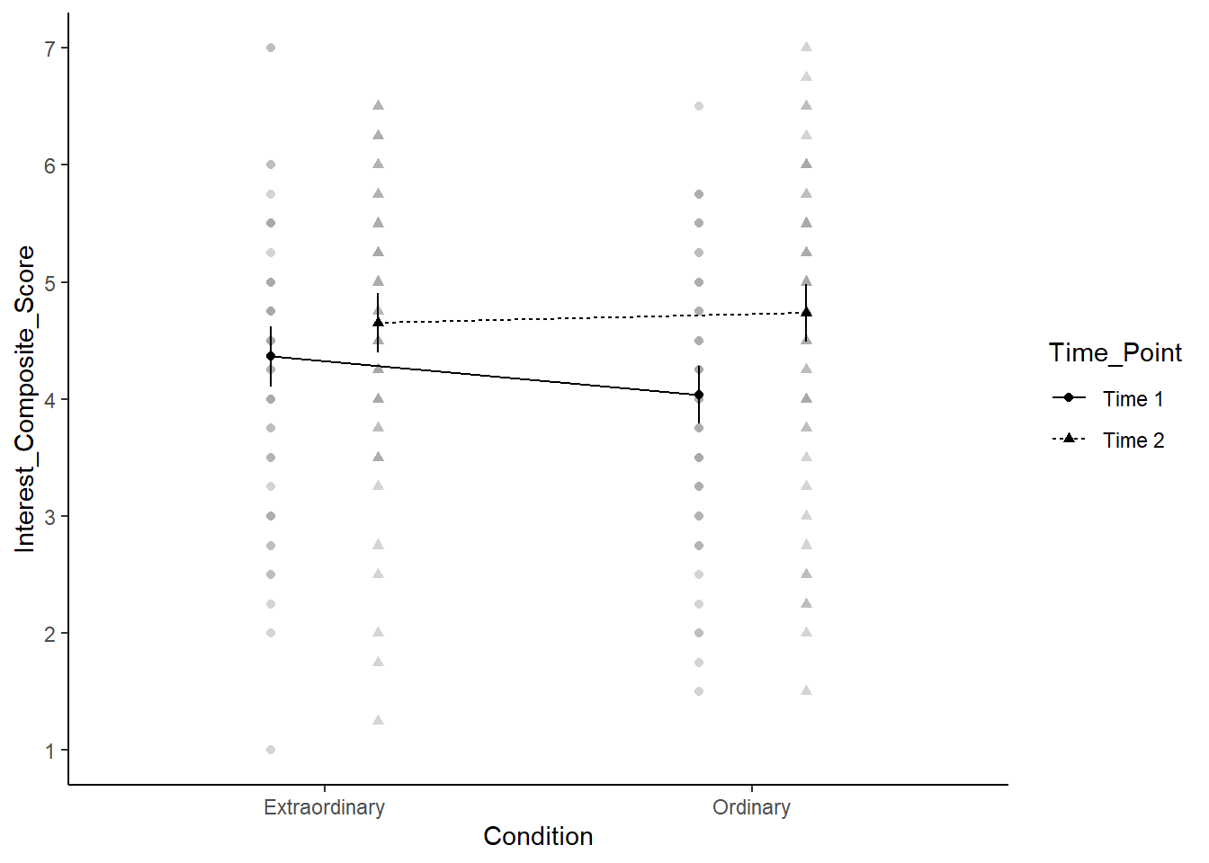

13.8.3 Effect sizes for each comparison

To calculate standardised effect sizes for the pairwise comparisons, we again need to do this individually using the cohens_d() function from the effectsize package. Here is where zhang_data is becoming useful.

As we have a mixed design, we must follow a slightly different process for each comparison. Cohen’s d has a different calculation for between-subjects and within-subjects contrasts, so we must express it differently.

For the first comparison, we are interested in the difference between time 1 and time 2 for each group, so this represents a within-subjects comparison.

# time 1 vs time 2 for Extraordinary group
cohens_d(x = "Time 1", 
         y = "Time 2", 
         paired = TRUE,
         data = filter(zhang_data, 
                       Condition == "Extraordinary"))

For paired samples, 'repeated_measures_d()' provides more options.

Cohens_d	CI	CI_low	CI_high
-0.3086922	0.95	-0.554559	-0.0605597

# time 1 vs time 2 for Ordinary group
cohens_d(x = "Time 1", 
         y = "Time 2", 
         paired = TRUE,
         data = filter(zhang_data,
                       Condition == "Ordinary"))

For paired samples, 'repeated_measures_d()' provides more options.

Cohens_d	CI	CI_low	CI_high
-0.5552045	0.95	-0.816696	-0.2898832

For the second comparison, we are interested in the difference between ordinary and extraordinary at each time point, so this represents a between-subjects comparison.

# Extraordinary vs ordinary at time 1
cohens_d(`Time 1` ~ Condition,
         data = zhang_data)

Cohens_d	CI	CI_low	CI_high
0.2914024	0.95	-0.0548458	0.6365251

# Extraordinary vs ordinary at time 2
cohens_d(`Time 2` ~ Condition,
         data = zhang_data)

Cohens_d	CI	CI_low	CI_high
-0.0695901	0.95	-0.413401	0.2744922

13.9 Activity 9: The write-up

We can now replicate the write-up paragraph from the paper. However, note we report t-test for the post hoc comparison (tbh, I have no clue why Zhang et al. decided on ANOVAs reporting when there is only 2 levels to compare):

We conducted the same repeated measures ANOVA with interest as the dependent measure and again found a main effect of time, \(F(1, 128) = 25.88, p < .001, η_p^2 = 0.168\); anticipated interest at Time 1 \((M = 4.20, SD = 1.12, 95\% CI = [4.01, 4.39])\) was lower than actual interest at Time 2 \((M = 4.69, SD = 1.19, 95\% CI = [4.49, 4.90])\).

We also observed an interaction between time and type of experience, \(F(1, 128) = 4.45, p = .037, η_p^2 = 0.034\). Pairwise comparisons revealed that for ordinary events, predicted interest at Time 1 \((M = 4.04, SD = 1.09, 95\% CI = [3.76, 4.31])\) was lower than experienced interest at Time 2 \((M = 4.73, SD = 1.24, 95\% CI = [4.44, 5.03])\), \(t(128) = -5.05, p < .001, d = -0.56\). Although predicted interest for extraordinary events at Time 1 \((M = 4.36, SD = 1.13, 95\% CI = [4.09, 4.63])\) was lower than experienced interest at Time 2 \((M = 4.65, SD = 1.14, 95\% CI = [4.36, 4.94])\), \(t(128) = -2.12, p = .036, d = -0.31\), the magnitude of underestimation was smaller than for ordinary events.

Pair-coding

to be added

Test your knowledge

Question 1

A researcher wants to compare memory test scores across three different age groups (young adults, middle-aged adults, and older adults). What type of ANOVA should they use?

One-way between-subjects ANOVAOne-way repeated-measures ANOVAFactorial ANOVAMixed factorial ANOVA

Explain this answer

Correct Answer:

A one-way between-subjects ANOVA is appropriate because there is one independent variable (age group) with three levels, and each participant is only tested in one group.

Incorrect Answers:

A One-way repeated-measures ANOVA is incorrect because it is used when the same participants are measured multiple times. Here, participants can only be allocated to one group.
A Factorial ANOVA is incorrect because it is used when there are two or more independent variables.
A mixed factorial ANOVA is incorrect because it is used when there is at least one between-subjects factor and one within-subjects factor.

Question 2

A researcher investigates how type of social media use (Passive, Active–Personal, Active–Public) and time of day (Morning vs Evening) affect self-esteem. They run a 3 × 2 mixed factorial ANOVA and follow up a significant interaction using emmeans() with pairwise comparisons at each level of the other variable.

Below is a partial output of the post hoc tests:

Contrasts of Time_Point at each Condition

# emmeans(mod, ~ Time_Point * Condition) %>%
#   contrast(interaction = "pairwise", simple = "each", combine = FALSE)


# === Passive Users ===
contrast               estimate   SE    df  t.ratio   p.value
Morning - Evening        2.00    0.31   48   -6.45     <.001

# === Active–Personal Users ===
contrast               estimate   SE    df  t.ratio   p.value
Morning - Evening       -2.50    0.32   48   -7.81     <.001

# === Active–Public Users ===
contrast               estimate   SE    df  t.ratio   p.value
Morning - Evening       -1.00    0.31   48   -3.23     0.005

Which of the following statements best reflects these findings?

Only Active users show significant changes in self-esteem over time.You cannot see the directionality of the comparison from the output, only that there is a significant difference.Self-esteem increased over the day in all three groups.Passive users showed a drop in self-esteem across the day, while both active user groups showed increases.

Explain this answer

Correct Answer: Passive users showed a drop in self-esteem across the day, while both active user groups showed increases.

The contrast is Morning - Evening, so a positive estimate means Morning scores were higher than Evening scores (i.e., a drop across the day). Passive users show a positive value (2.00), while both Active-Personal (−2.50) and Active-Public (−1.00) show negative values, indicating higher self-esteem in the evening (i.e., an increase across the day).

Incorrect Answers:

Self-esteem increased over the day in all three groups.: Only the active user groups showed an increase (negative estimates = Evening > Morning). Passive users actually showed a decrease in self-esteem (positive estimate = Morning > Evening).
Only Active users show significant changes in self-esteem over time.: All three groups show statistically significant changes (p < .05), including Passive users. The difference lies in the direction of change—not whether a change occurred.
You cannot see the directionality of the comparison from the output, only that there is a significant difference.: The direction is clearly shown by the estimate: positive means higher in the Morning, negative means higher in the Evening. This output lets you interpret both the presence and direction of the effect.

Question 3

Which of the following is the most appropriate method for checking whether the residuals in a mixed factorial ANOVA are normally distributed?

Visually inspect the spread of data points using a bar chartUse Levene’s Test to compare variance across groupsCheck whether the independent variable is normally distributed in each conditionGenerate a Q–Q plot of residuals

Explain this answer

Correct Answer:

Generate a Q–Q plot of residuals is correct because this visual tool helps assess whether the residuals follow a normal distribution.

Incorrect Answers:

Use Levene’s Test to compare variance across groups is incorrect as this checks for homogeneity of variance, not normality.
Check whether the independent variable is normally distributed in each condition is incorrect because ANOVA assumes that the residuals of the dependent variable, not the independent variable, are normally distributed. The IV is usually categorical and doesn’t require normality.
Visually inspect the spread of data points using a bar chart is incorrect since bar charts show averages, not the distribution of residuals.

Question 4

You run a 3 × 4 mixed factorial ANOVA and find a significant interaction. What is the most appropriate next step?

Rerun the analysis using a one-way ANOVA for each groupInterpret only the main effects of each factorIgnore the interaction since it complicates the interpretationConduct post hoc comparisons to explore simple effects

Explain this answer

Correct Answer:

Conduct post hoc comparisons to explore simple effects is correct because a significant interaction suggests that the effect of one factor depends on the level of the other. To fully understand this, you need to explore the simple effects, i.e., how one variable behaves at each level of the other.

Incorrect Answers:

Interpret only the main effects of each factor is incorrect because a significant interaction indicates that the effect of one factor depends on the level of the other. Interpreting main effects alone would be misleading.
Rerun the analysis using a one-way ANOVA for each group is incorrect as this would ignore the factorial structure and inflate the risk of Type I error. The proper approach is to follow up the interaction with simple effects comparisons, not separate one-way ANOVAs.
Ignore the interaction since it complicates the interpretation is incorrect because the interaction is a meaningful result. Ignoring it would overlook important patterns in the data and lead to an incomplete or inaccurate interpretation.