Lab 12 Continuing the GLM: One-factor ANOVA
12.1 Overview
In the previous chapter you learned how to decompose a dependent variable into components of the general linear model, expressing the values in terms of a decomposition matrix, before finishing up with calculating the sums of squares. In this chapter, we will take it a step further and look at running the ANOVA from those values. Through this we will start exploring the relationships between sums of squares (SS), mean squares (MS), degrees of freedom (df), and F-ratios. In this chapter we will show you how you go from the decomposition matrix we created in the previous chapter to actually determining if there is a significant difference or not.
In the last chapter we had you work through the calculations step-by-step "by hand" to gain a conceptual understanding, and we will continue that in the first half of the inclass activities. However, when you run an ANOVA, typically the software does all of these calculations for you. As such, in the second part of the activities, we'll show you how to run a one-factor ANOVA using the aov_ez() function in the afex add-on package. From there you will see how the output of this function maps onto the concepts you've been learning about.
Some key terms from this chapter are:
- Sums of Squares (SS) - an estimate of the total spread of the data (variance) around a parameter (such as the mean). We saw these in Chapter 11
- degrees of freedom (df) - the number of observations that are free to vary to produce a known output. Again we have seen these before in all previous tests. The df impacts on the distribution that is used to compare against for probability
- Mean Square (MS) - an average estimate of the spread of the data (variance) calculated by \(MS = \frac{SS}{df}\)
- F-ratio - the test statistic of the ANOVA from the F-distribution. Calculated as \(F = \frac{MS_{between}}{MS_{within}}\) or \(F = \frac{MS_{A}}{MS_{err}}\).
Again, these terms will become more familiar as we work through this Chapter so don't worry if you don't understand them yet. The main thing to understand is that we go from the indivual data to the decomposition matrix to the Sums of Squares to the Mean Squares to the F-ratio. But in summary this is what we are doing:
ANOVA PATH: \(Data \to Decomp. Matrix \to SS \to MS \to F\)
As such, the goals of this chapter are to:
- to demonstrate how Sums of Squares leads to an F-value, finishing off the decomposition matrix
- to determine the probability of a F-value for given degrees of freedom (df)
- to explore using the
aov_ez()function and how the outcome compares to your decomposition matrix calculations.
Note: The afex package is already installed on the Boyd Orr machines and only needs read into the library in the normal fashion. Do not install it on the Boyd Orr Lab machines. If you are using your own laptop you will need to make sure you have installed the afex package.
12.2 PreClass Activity
As per the previous Chapter, the PreClass activity for this lab is reading (re-reading in fact) and trying out some of the Miller and Haden activities. We will go over similar activities in the remainder of this chapter so it will really help you to spend a few minutes trying out the Miller and Haden activities and thinking about them.
12.2.1 Read
Chapters
- Re-read Chapter 3 of Miller and Haden (2013) and make sure you are understanding it. Particularly focus on how the decomposition matrix leads to the ANOVA output through sums of squares, dfs, and mean squares.
12.2.2 Try
Activities
- Test your understanding by working through Computational Exercise #1 in section 3.12 of Miller and Haden (page 31) all the way to the summary table. The answer is in Miller and Haden section 3.13 but be sure to work through the example first. Don't worry about sketching the data. What you want to do is work the values through the decomposition matrix all the way to the F-value.
- The decomposition matrix is very similar to the one we looked at in Chapter 11, but with less conditions.
- The sums of squares would be calculated the same way as we did in Chapter 11.
- Use the formulas shown to calculate F.
\[MS = \frac{SS}{df} \space\space\space\space\space F = \frac{MS_{between}}{MS_{within}}\]
- It may also help to review Chapter 4 on probability as we move onto understanding F distributions and p-values.
Job Done - Activity Complete!
12.3 InClass Activity
One-factor ANOVA: Worked example
Just like we did in Chapter 11, let's start with some simulated data corresponding to a between-subjects design with three groups (conditions/levels) on one factor (variable). In this hypothetical study, you're investigating the effects of ambient noise on concentration. You have participants transcribe a handwritten document onto a laptop and count the number of typing errors (DV = typos) each participant makes under their respective different conditions:
- while hearing ambient conversation such as you would find in a busy cafe (cafe condition);
- while listening to mellow jazz music (jazz condition);
- or in silence (silence condition).
Again for practice we will only use small, highly under-powered groups. You have three different participants in each condition. As such, your data are as follows:
- cafe: 111, 102, 111
- jazz: 89, 127, 90
- silence: 97, 85, 88
Below is the decomposition matrix for this data set, based on the GLM: \[Y_{ij} = \mu + A_i + S(A)_{ij}\]
Here we are copying what we did in the last chapter in both the inclass and assignment and what you did for the homework activity - with just less participants. You can have a go at creating the decomposition matrix yourself from scratch if you like, as good practice, or, in the interests of time, feel free to reveal the code and run that code to create the dmx.
Note that we have also included a column called sub_id with a unique identifier for each participant. This is not that important for the decomposition matrix but we will definitely need it later for running the ANOVA using the afex::aov_ez() function, so let's just include it now so we don't forget.
dmx <- tibble(sub_id = 1:9,
              i = rep(1:3, each = 3),
              j = rep(1:3, times = 3),
              typos = c(111, 102, 111,
                    89, 127, 90,
                    97, 85, 88),
              sound = rep(c("cafe", "jazz", "silence"), each = 3)) %>%
  mutate(mu = mean(typos)) %>%
  group_by(i) %>%
  mutate(Ai = mean(typos) - mu) %>%
  ungroup() %>%
mutate(err = typos - (mu + Ai))| sub_id | i | j | typos | sound | mu | Ai | err |
|---|---|---|---|---|---|---|---|
| 1 | 1 | 1 | 111 | cafe | 100 | 8 | 3 |
| 2 | 1 | 2 | 102 | cafe | 100 | 8 | -6 |
| 3 | 1 | 3 | 111 | cafe | 100 | 8 | 3 |
| 4 | 2 | 1 | 89 | jazz | 100 | 2 | -13 |
| 5 | 2 | 2 | 127 | jazz | 100 | 2 | 25 |
| 6 | 2 | 3 | 90 | jazz | 100 | 2 | -12 |
| 7 | 3 | 1 | 97 | silence | 100 | -10 | 7 |
| 8 | 3 | 2 | 85 | silence | 100 | -10 | -5 |
| 9 | 3 | 3 | 88 | silence | 100 | -10 | -2 |
We finished off last week by calculating the Sums of Squares for the different columns - a measure of the variance attributable to that part of the model (or that column). Remember that to calculate the Sums of Squares (or often shortend to \(SS\)) we square all the values in a column and sum them up. So for example:
\[SS_{\mu} = \sum\mu^2 = (\mu_{11} \times \mu_{11}) + (\mu_{12} \times \mu_{12}) + \space ... \space (\mu_{33} \times \mu_{33})\]
We also said at the end of the last Chapter that the Sums of Squares of the different columns were all linked through the following relationship:
\[SS_{total} = SS_{\mu} + SS_{A} + SS_{error}\]
- Have a go at calculating the SS of the above decomposition matrix (
dmx) using the code we showed you towards the end of the inclass activity in the last chapter. If unsure, then the code can be revealed below:
dat_ss <- dmx %>%
  summarise(total = sum(typos^2),
            ss_mu = sum(mu^2),
            ss_sound = sum(Ai^2),
ss_err = sum(err^2))- Which would give:
| total | ss_mu | ss_sound | ss_err |
|---|---|---|---|
| 91574 | 90000 | 504 | 1070 |
We can then check that we have calculated everything correctly by using the following relationship:
\[SS_{total} = SS_{\mu} + SS_{A} + SS_{error}\]
then:
\[91574 = 90000 + 504 + 1070\]
12.3.1 Task 1 - Quick Checks
QuickFire Questions
Answer the following questions. The solutions are at the end of the chapter.
If the corrected total Sum of Squares is the \(SS_{total}\) minus the part of the total attributable to the intercept (i.e., the grand mean, \(SS_{\mu}\)), calculate the corrected total Sum of Squares for the above example.
- hint: \(SS_{corrected} = SS_{total} - SS_{\mu}\)
What proportion of the corrected total sum of squares is attributable to the main effect of
sound?- hint: \(SS_{sound} = SS_{A}\)
- hint: \(\frac{SS_{sound}}{SS_{corrected}}\)
What proportion of the corrected total sum of squares is attributable to residual error?
- hint: \(SS_{error}\)
12.3.2 Task 2 - Mean squares and degrees of freedom
Great, so now we know how to create our decomposition matrix and how to calculate our sums of squares. The only thing left to do is to calculate the F-ratio (the test statistic for the ANOVA, otherwise called the F-value) to determine if there is a significant effect between our groups. But, as it is always good to have a view of the whole picture, let's not forget that the whole purpose here is to show you where the numbers come from in our quest to determine if there is a significant difference between our groups, or in other words, is there an effect of listening condition on concentration!
You will remember from your lectures and from your reading of Miller & Haden (2013) that the F-value is a ratio of two estimates of population variance:
\[F = \frac{MS_{between}}{MS_{within}} = \frac{MS_{treatment}}{MS_{error}} = \frac{MS_{A}}{MS_{S(A)}}= \frac{MS_{A}}{MS_{error}}\]
And you will also remember that the Mean Square (MS) is the Sums of Squares (SS) divided by its degrees of freedom (df). If you don't remember what degrees of freedom are, go back to pages 21-23 of Miller and Haden (2013). They have a good explanation for it, however, these things are easy to forget, so make sure to qucikly skim back through the book. So the general formula for the Mean Square is:
\[MS = \frac{SS}{df}\]
Let's start trying to put all this information together! If we know the SS of our group/treatment (\(SS_{A} = 504\) - also called the between variance) and we know the SS of our error/residuals (\(SS_{error} = 1070\) - also called the within variance), then we can convert both of the \(SS\)s to Mean Squares (MS) (i.e. the average variance for that condition) by dividing them by their respective degrees of freedom (df).
We can then calculate F-value (also called F-observed) by: \[F = \frac{MS_{A}}{MS_{error}}\]
If the \(MS_{error}\) is larger than \(MS_{A}\) (the group effect) then F-value will be small and there will be no significant effect of group - any difference in groups is purely due to individual differences (another way of thinking about error). On the other hand, if \(MS_{A}\) (the group effect) is larger than \(MS_{error}\) then F-value will be large, and depending on how large the F-value is, there may be a significant difference caused by your group variable.
With all that in mind, and it may take a couple of readings, try to answer the following questions (consulting Miller & Haden Ch. 3 and your lecture slides where needed). The solutions are at the end of the chapter.
QuickFire Questions
- Stated in terms of \(\mu_{jazz}\), \(\mu_{cafe}\), and \(\mu_{silence}\), what is the null hypothesis for this specific study of the effects of sound on typographic errors? You may need to look back to Chapters 6 and 7 to think about this.
Hint: the alternative hypothesis for a two condition experiment would be \(\mu_{1} \ne \mu_{2}\)
How many degrees of freedom are there for \(A_{i}\), the main effect of sound, if \(dfA_{i}\) = k - 1?
How many degrees of freedom are there for \(S(A)_{ij}\), the error term, if \(dfS(A)_{ij}\) = N - \(dfA_{i}\) - 1?
Hint: You can also refer to \(dfS(A)_{ij}\) as \(df_{error}\)
- Calculate \(MS_{A}\), where \(A\) is the factor sound.
Note: You can access individual columns in a table using double square brackets [[]]; for instance dat_ss[["ss_mu"]] gives you the column ss_mu from dat_ss. This is an alternative to $ that some may know; e.g. dat_ss$mu.
- Calculate \(MS_{S(A)}\).
Hint: You can also refer to \(MS_{S(A)}\) as \(MS_{error}\)
- Remember that the null says that there are no differences between conditions.
- Sound, our factor, has three levels.
- N is the total number of participants
- \(MS_{A} = \frac{SS_{A}}{dfA_{i}}\)
- \(MS_{S(A)} = \frac{SS_{error}}{dfS(A)_{ij}}\)
12.3.3 Task 3 - F-ratios
Last step, calculating the F-value. As above, if the null hypothesis is true (\(\mu_{1} = \mu_{2} = \mu_{3}\)), then both estimates of the population variance (\(MS_{between}\) and \(MS_{within}\)) should be equal, and the \(F\)-ratio should approach 1 (because \(\frac{x}{x} = 1\)). Now, we can't expect these two estimates to be exactly equal because of sampling bias, so to see how unlikely our observed F-ratio is under the null hypothesis, we have to compare it to the F-distribution.
To learn a bit about the F-distribution we have created a shiny app to play with, which you can see below. Shiny Apps are interactive webpages and applications made through R.
Figure 4.12: F-distribution app
The F distribution is a representation of the probability of various values of F under the null hypothesis. It depends upon two parameters: \(df_{numerator}\) and \(df_{denominator}\). Play around with the sliders corresponding to these two parameters and observe how the shape of the distribution changes.
There is also a slider that lets you specify an observed \(F\) ratio (to one digit of precision). It is represented on the blue line of the graph. Move this slider around and watch how the p-values change. The p-value is the total area under the curve to the right of the blue line.
The red line on the plot denotes the critical value of F required for a significant difference, given the \(\alpha\) (type 1 error rate) and the \(df_{numerator}\) and \(df_{denominator}\) .
QuickFire Questions
Try using your data and the app to answer the following questions. The solutions are at the end of the chapter.
From your data, calculate the observed F-value (called
f_obs) for the effect ofsoundontypos(concentration).- hint: \(MS_{between} / MS_{within}\)
Using the app shown above, set \(\alpha = .05\), set the degrees of freedom to correspond to those in your study, and set the observed F ratio as close as you can to the value you got in the above question.
Now, according to the app, what is the critical value for \(F\) (hint: red line)?
According to the app, what is the approximate \(p\) value associated with your observed \(F\) ratio?
Based on these values, do you reject or retain the null hypothesis?
Tricky question: Note that you can use the distribution functions for \(F\) in the same way you did in Chapter 4 for the normal distribution (pnorm(), dnorm(), qnorm()) or for the binomial distribution (pbinom(), dbinom(), qbinom()), keeping in mind however that the F distribution, being continuous, is more analogous to the normal distribution. See ?df for the distribution functions associated with \(F\).
- Using the appropriate distribution function, calculate the \(p\) value associated with \(F_{obs}\). This will be more precise than the app.
- look at inputs for the function - ?pf
- ignore ncp
- f_obs = q
- lower.tail? What is the probability of obtaining an F_obs higher than your value.
12.3.4 Task 4 - Using afex::aov_ez()
Great, so we have calculated the F-value for this test and made a judgement about whether it is significant or not. But that was quite a long way of doing it, and whilst it is always great to understand where the data comes from, you don't want to have to do that each time you run a test. So now we are going to re-analyse the same dataset but this time we are going to have the computer do all the computational work for us.
There are various options for running ANOVAs in R, but the function we will be using for this course is aov_ez() function in the afex add-on package. Note that to use aov_ez() you either have to load in the package using library(afex), or you can call it directly without loading using afex::aov_ez() (the package_name::function syntax). If you're just using the function once, the latter often makes more sense. The afex package is already installed in the Boyd Orr machines so it only needs called to the library. On your own machines you will need to install the package if you haven't already done so.
- Have a quick read through the documentation for
aov_ez(type?aov_ezin the console) and then look at the code below which shows how to run the ANOVA and try to understand it. Pay specific attention to how you stipulate the datafile, the dv, the factor, the participants, etc.
library(afex)

dat <- select(dmx, sub_id, typos, sound)

results <- afex::aov_ez(data = dat,
                         dv = "typos",
                         id = "sub_id",
                         type = 3,
                         between = "sound")
You will have seen a couple of messages pop up about converting sound to factor. That is fine. You can see these in the solutions if you want to confirm yours are the same. If we then look at the output of the analysis through the following code:
print(results$Anova)We see:
## Anova Table (Type III tests)
##
## Response: dv
##             Sum Sq Df  F value    Pr(>F)
## (Intercept)  90000  1 504.6729 5.091e-07 ***
## sound          504  2   1.4131    0.3142
## Residuals     1070  6
## ---
## Signif. codes:  0 '***' 0.001 '**' 0.01 '*' 0.05 '.' 0.1 ' ' 1
And if you ran the following code:
print(results$anova_table)Then you would be able to see the effect size for this ANOVA in the form of generalised eta-squared (ges) - \(\eta_G^2 = .32\):
## Anova Table (Type 3 tests)
##
## Response: typos
##       num Df den Df    MSE      F    ges Pr(>F)
## sound 2 6 178.33 1.4131 0.3202 0.3142- Looking at the ANOVA ouput, do you see how the numbers match up with what we calculated above? You can ignore the intercept for now (though the Sums of Squares will be familiar). This table doesn't show the Mean Squares but it does show the Sums of Squares and the F-value.
- What do you conclude about the effects of ambient noise on concentration?
Conclusion
Not much to be honest with you! The study returns a non-significant finding suggesting that there is no significant effect of ambient noise on concentration, F(2, 6) = 1.413, p = .31, ges = 0.32. However, before you go off and publish this highly underpowered study we should probably look to replicate it with a larger sample (which you could calculate using your skills from Chapter 8).
Job Done - Activity Complete!
Excellent work today! And super interesting as well, huh? Quick, everyone to the cafe and don't worry about the typos!!!! Only joking, we are all going to the cafe to replicate!
One last thing:
Before ending this section, if you have any questions, please post them on the available forums or speak to a member of the team. Finally, don't forget to add any useful information to your Portfolio before you leave it too long and forget. Remember the more you work with knowledge and skills the easier they become.
12.4 Assignment
This is a summative assignment and as such, as well as testing your knowledge, skills, and learning, this assignment contributes to your overall grade for this semester. You will be instructed by the Course Lead on Moodle as to when you will receive this assignment, as well as given full instructions as to how to access and submit the assignment. Please check the information and schedule on the Level 2 Moodle page.
12.5 Solutions to Questions
Below you will find the solutions to the questions for the Activities for this chapter. Only look at them after giving the questions a good try and speaking to the tutor about any issues.
12.5.1 InClass Activities
12.5.1.1 InClass Task 1
Question 1
- \(SS_{corrected\ total} = SS_{total} - SS_{\mu}\)
- \(SS_{total}\) = 91574
- \(SS_{\mu}\) = 90000
- \(SS_{corrected\ total}\) = 91574 - 90000 = 1574
Question 2
- \(SS_{sound}\) = 504
- \(SS_{corrected\ total}\) = 1574
- \(SS_{sound} / SS_{corrected\ total}\) = 504 / 1574 = 0.32
Question 3
- \(SS_{err}\) = 1070
- \(SS_{corrected\ total}\) = 1574
- \(SS_{err} / SS_{corrected\ total}\) = 1070 / 1574 = 0.68
12.5.1.2 InClass Task 2
Question 1
\(\mu_{cafe} = \mu_{jazz} = \mu_{silence}\)
Question 2
- k = number of conditions, so:
df = k - 1 = 3 - 1 = 2
Question 3
- N = 9, and \(dfA_{i}\) = 2, so
df = 9 - 2 - 1 = 6
Question 4
- The factor df = 2
ms_a <- dat_ss[["ss_sound"]] / 2L- Giving \(MS_{A}\) = 252
Question 5
- The residual df = 6
ms_err <- dat_ss[["ss_err"]] / 6L- Giving \(MS_{S(A)}\) = 178.3333333
12.5.1.3 InClass Task 3
Question 1
f_obs <- ms_a / ms_err- Giving a F-value of F = 1.413 when rounded to three decimal places.
Question 2
The red line should be about F = 5.143, meaning that that is the minimum value of F, for those dfs, considered to be statistically significant at \(\alpha = .05\)
Question 3
Reading off the app, the approximate p-value for f_obs is p = .317.
Question 4
As \(p\) > \(\alpha\) we would retain the null hypothesis that there is no significant effect of group in this study
Question 5
This could alternatively calculated using coding as such:
pf(f_obs, 2, 6, lower.tail = FALSE)Which would give a p-value of p = 0.314 and again could be written up as F(2, 6) = 1.413, p = 0.314, suggesting no significant effect of ambiance or location on concentration as measured through the number of typos.
12.5.1.4 InClass Task 4
dat <- select(dmx, sub_id, typos, sound)

results <- afex::aov_ez(data = dat,
                         dv = "typos",
                         id = "sub_id",
                         type = 3,
                         between = "sound")
## Registered S3 methods overwritten by 'lme4':
## method from
## cooks.distance.influence.merMod car
## influence.merMod car
## dfbeta.influence.merMod car
## dfbetas.influence.merMod car## Converting to factor: sound## Contrasts set to contr.sum for the following variables: sound
And when we look at the output table see:
| Sum Sq | Df | F value | Pr(>F) | |
|---|---|---|---|---|
| (Intercept) | 90000 | 1 | 504.673 | 0.000 |
| sound | 504 | 2 | 1.413 | 0.314 |
| Residuals | 1070 | 6 |
From this we can see that the numbers we calculated match up exactly with the values that the function produced - F(2, 6) = 1.41, p = .31. You can also see that there is no significant effect and as such we cannot reject the null hypothesis.
Chapter Complete!
12.6 Additional Material
Below is some additional material that might help you understand ANOVAs a bit more and some additional ideas.
12.6.1 Levene's Test of Homogeneity
From previous chapters and from your lectures you will know that every test has a series of assumptions that are required to be held in order for your conclusions to be valid, and the ANOVA is no exception. As always the specific assumptions change depending on the design of the study, but in the instance of the experiment in this chapter - a between-subjects design - the assumptions are as follows:
- Data should be interval/ratio
- Data in each condition should be normally distributed
- Data is independent from each other
- There is homogeneity of variance across different conditions (i.e. different conditions have equal variances).
You will spot that these are actually very similar to a between-subjects t-test and that again just shows that the two tests are highly related.
Now we know various ways to check things like normality and variance, with visual inspection being one of them, but a common test that people tend to use is what is called Levene's Test of Homogeneity. In fact, if you think back to Chapter 7, when you run a t-test and set the variance as var.equal = FALSE, if you really wanted to run the test as var.equal = TRUE then it would be Levene's test you should run first to confirm that variance is actually equal. However, the issue with the ANOVA is that it actually assumes variance is equal, so it is best to run a Levene's test whenever you run an ANOVA that has at least one between-subjects condition. That is what we are going to show you here as well as how to interpret it and a little bit of discussion after. The main thing to note about Levene's Test of Homogeniety is that the null hypothesis for this test states that there is no significant difference in variance between conditions:
\[H_{0}: \sigma_{1}^2 = \sigma_{2}^2 \] Conversely, the alternative hypothesis states that there is a difference in variance between conditions:
\[H_{1}: \sigma_{1}^2 \ne \sigma_{2}^2 \]
So a non-significant finding in Levene’s test would suggests equal variance across conditions as required by the assumptions of the ANOVA, whereas a significant finding for Levene's Test would suggest unequal variance and you may need to think about the assumptions of your data.
Running the test
So here is our data again from the main activities, which we have stored in a tibble calleddmx:
| sub_id | i | j | typos | sound | mu | Ai | err |
|---|---|---|---|---|---|---|---|
| 1 | 1 | 1 | 111 | cafe | 100 | 8 | 3 |
| 2 | 1 | 2 | 102 | cafe | 100 | 8 | -6 |
| 3 | 1 | 3 | 111 | cafe | 100 | 8 | 3 |
| 4 | 2 | 1 | 89 | jazz | 100 | 2 | -13 |
| 5 | 2 | 2 | 127 | jazz | 100 | 2 | 25 |
| 6 | 2 | 3 | 90 | jazz | 100 | 2 | -12 |
| 7 | 3 | 1 | 97 | silence | 100 | -10 | 7 |
| 8 | 3 | 2 | 85 | silence | 100 | -10 | -5 |
| 9 | 3 | 3 | 88 | silence | 100 | -10 | -2 |
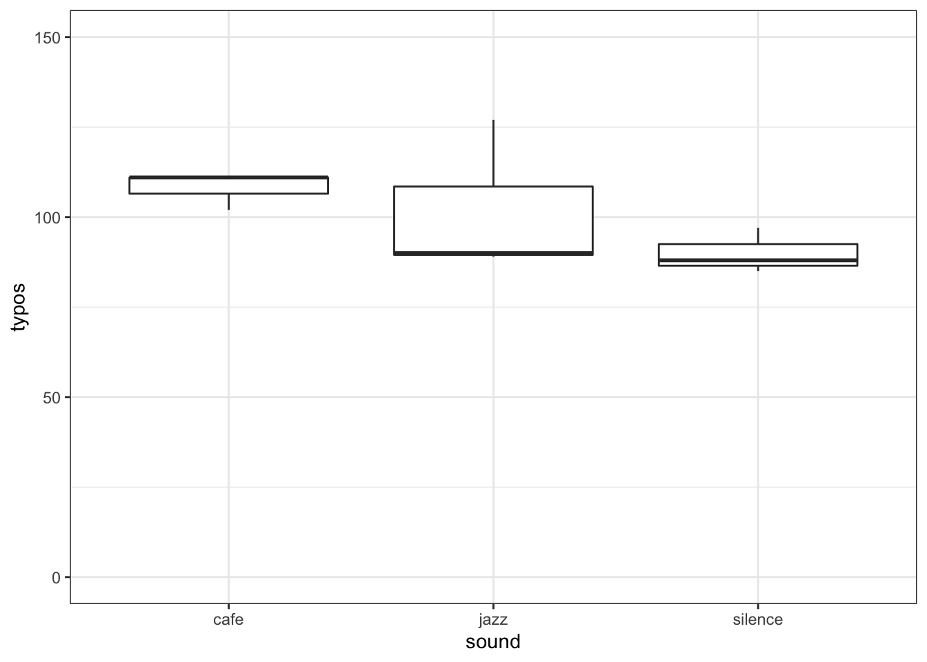
Figure 12.1: A boxplot of our data to check for homogeneity of variance
And as you can see it does not look like there is equal variance. However, maybe we don't really trust our eyes and as such we want to run the Levene's Test. To do that we use the below code:
car::leveneTest(typos ~ sound, data = dmx, center = median)## Warning in leveneTest.default(y = y, group = group, ...): group coerced to
## factor.Where we are:
- using the
leveneTest()function from thecarpackage. - using the formula approach that we saw in t-test where we are saying effectively DV "by" IV - typos ~ sound, where
~stands for "by".
- saying the data is in the tibble
dmx - and we are telling the code to run based on the medians of the distribution. This is a bit of a judgement call and you could use the mean instead of the median, but this paper would seem to suggest the median is optimal: Carroll & Schnieder (1985) A note on levene's tests for equality of variances
If we run the leveneTest() code we get the following output:
## Warning in leveneTest.default(y = y, group = group, ...): group coerced to
## factor.| Df | F value | Pr(>F) | |
|---|---|---|---|
| group | 2 | 0.5165877 | 0.6208682 |
| 6 | NA | NA |
And now with your knowledge of understanding F-values and ANOVA tables (see Levene's is really just a sort of ANOVA) you can determine that, F(2, 6) = 0.517, p = .621. This tells us that there is no significant difference between the variance across the different conditions. Which, if you look at the boxplot, is completely the opposite of what we expected! Why is that? Most likely, that is because we have such small numbers of participants in our samples and you will remember from Chapter 8, small samples mean low power and unreliable findings. This is actually a good example why people often use visual inspection as well as some analytical tests to make checks on assumptions and they pull information together to make a judgement. The boxplot would say that variance is unequal. Levene's test would say variance is equal. Here, I would probably suggest taking a cautious approach and run a lot more participants before I consider running my analysis.
Using afex to run Levene's
One issue with the above example is that it requires another package - car. This isn't a major problem but say you only had the afex package to use. Well fortunately that package also has a function that can check Levene's Test - afex::test_levene(). And it works as follows:
- First run the ANOVA as shown in the chapter and store the output
results <- afex::aov_ez(data = dmx,
                         dv = "typos",
                         id = "sub_id",
                         type = 3,
                         between = "sound")
## Registered S3 methods overwritten by 'lme4':
## method from
## cooks.distance.influence.merMod car
## influence.merMod car
## dfbeta.influence.merMod car
## dfbetas.influence.merMod car## Converting to factor: sound## Contrasts set to contr.sum for the following variables: sound- Now use the output of the ANOVA, in this instance
results, as the input for the Levene's Test, and again center on the median
afex::test_levene(results, center = median)| Df | F value | Pr(>F) | |
|---|---|---|---|
| group | 2 | 0.5165877 | 0.6208682 |
| 6 | NA | NA |
And if we look at that output we see the exact same finding as we did using car::leveneTest()- F(2, 6) = 0.517, p = .621. So the positives of this approach is that you only use one package and it gives the same results as using two packages. The downside is that you have to run the ANOVA first - see how we use the ANOVA output as an input for test_levene() - which is a bit of an odd way of treating this assumption. Normally you would run the assumption check first and then the test.
Help I have unequal variance!
Right, so you have found that your variance is not equal and you are now worried about what to do in regards your assumptions. Well, there is much debate on how robust the ANOVA is, where robust would mean that your False Positive rate does not necessarily inflate if the assumptions are not held. Some say that the ANOVA is not robust and you should use a non-parametric style of analysis instead in this instance, or break the ANOVA down into a series of Welch's t-tests (assuming unequal variance) and control the False Positive rate through Bonferroni corrections. Some however say that the ANOVA is actually pretty robust. We would recommend reading this paper Blanca et al. (2018) Effect of variance ratio on ANOVA robustness: Might 1.5 be the limit? which suggests that some degree of unequal variance is acceptable. Alternatively, just as there is a Welch's t-test that does not assume equal variance there is also a Welch's ANOVA that does not assume equal variance. This paper Delacre et al., (preprint) Taking Parametric Assumptions Seriously Arguments for the Use of Welch’s F-test instead of the Classical F-test in One-way ANOVA goes into great detail about why using Welch's ANOVA is always advisable. You may be wondering how do you run a Welch's ANOVA in R, yeah? That is a very good question that you should ask Phil to write about one day after he figures it out himself.
End of Additional Material!