Lab 14 Regression

14.1 Overview

For the past few weeks we have been looking at designs where you have categorical factors/variables and where you want to see whether there is an effect of a given factor or an interaction between two factors on a continuous DV. And we have looked at this through decomposition matrices and through the afex package and the aov_ez() function. We also briefly mentioned how this approach can be extrapolated into designs with more than two factors such as three-way ANOVAs (three factors) and larger, but also into within-subject designs where every participant sees every stimuli, and mixed-designs where you have at least one between and one within factor. We will look in-depth at these different types of designs next year.

Today, however, we want to start looking at predicting relationships from continuous variables through regression. You will already be familiar with many of the terms here from your lecture series. In addition, by looking at a practical example (relating to voice research) in the lab, and by reading about regression in Miller and Haden (2013) in the PreClass, it should start to become more concrete for you. Regression is still part of the GLM and eventually the goal will be to show you how to analyse designs that has both categorical and continuous variables as much of real data is made up like that. But for now we will just look at simple linear regression and multitple linear regression to make you more comfortable with carrying out and interpreting these analyses.

The goals of this chapter are to:

Introduce the concepts that underpin linear regression.
Demonstrate and practice carrying out and interpreting regression analysis with one or more predictor variables.
Demonstrate and practice being able to make predictions based on your regression model.

14.2 PreClass Activity

As in previous chapters, the PreClass activity is to read the following chapter from Miller and Haden (2013). You may also want to try reading Chapter 14 as well on Multiple Regression but really more to add to your understanding of the general goal, as opposed to the underlying computations. Finally, reviewing your lecture on Simple Linear and Multiple Linear Regression will really help your understanding of this lab.

14.2.1 Read

Chapter

Read Chapter 12 of Miller and Haden (2013) and try to understand the how the GLM applies to regression. The concept of regression will be familiar to you based on the stats lectures of this semester so some of the terms will just be recapping. Some will be an expansion of your understanding and basing the analysis in terms of the GLM.

Optional

Read Chapter 14 of Miller and Haden (2013). This covers Multiple Linear Regression. Again the concepts will be familiar to you from the lecture series and reading this chapter would be to enhance your overall understanding, not necessarily the underlying computations.

Job Done - Activity Complete!

14.3 InClass Activity

You have been reading about regression in Miller and Haden (2013) and have been looking at it in the lectures. Today, to help get a practical understanding of regression, you will be working with real data and using regression to explore the question of whether there is a relationship between voice acoustics and ratings of perceived trustworthiness.

The Voice

The prominent theory of voice production is the source-filter theory (Fant, 1960) which suggests that vocalisation is a two step process: air is pushed through the larynx (vocal chords) creating a vibration, i.e. the source, and this is then shaped and moulded into words and utterances as it passes through the neck, mouth and nose, and depending on the shape of those structures at any given time you produce different sounds, i.e. the filter. One common measure of the source is pitch (otherwise called Fundamental Frequency or F0 (pronounced "F-zero")) (Titze, 1994), which is a measure of the vibration of the vocal chords, in Hertz (Hz); males have on average a lower pitch than females for example. Likewise, one measure of the filter is called formant dispersion (measured again in Hz), and is effectively a measure of the length of someone's vocal tract (or neck). Height and neck length are suggested to be negatively correlated with formant dispersion, so tall people tend to have smaller formant dispersion. So all in, the sound of your voice is thought to give some indication of what you look like.

More recently, work has focussed on what the sound of your voice suggests about your personality. McAleer, Todorov and Belin (2014) suggested that vocal acoustics give a perception of your trustworthiness and dominance to others, regardless of whether or not it is accurate. One extension of this is that trust may be driven by malleable aspects of your voice (e.g. your pitch) but not so much by static aspects of your voice (e.g. your formant dispersion). Pitch is considered malleable because you can control the air being pushed through your vocal chords (though you have no conscious control of your vocal chords), whereas dispersion may be controlled by the structure of your throat which is much more rigid due to muscle, bone, and other things that keep your head attached. This idea of certain traits being driven by malleable features and others by static features was previously suggested by Oosterhof and Todorov (2008) and has been tested with some validation by Rezlescu, Penton, Walsh, Tsujimura, Scott and Banissy (2015).

So the research question today is: can vocal acoustics, namely pitch and formant dispersion, predict perceived trustworthiness from a person's voice? We will only look at male voices today, but you have the data for female voices as well should you wish to practice (note that in the field, tendency is to analyse male and female voices separately as they are effectively sexually dimorphic). As such, we hypothesise that a linear combination of pitch and dispersion will predict perceived vocal trustworthiness in male voices. This is what we will analyse.

Let's begin.

First, to run this analysis you will need to download the data from here. You will see in this folder that there are two datafiles:

voice_acoustics.csv - shows the VoiceID, the sex of voice, and the pitch and dispersion values
voice_ratings.csv - shows the VoiceID and the ratings of each voice by 28 participants on a scale of 1 to 9 where 9 was extremely trustworthy and 1 was extremely untrustworthy

Have a look at the layout of the data and familiarise yourself with it. The ratings data is rather messy and in a different layout to the acoustics but can you tell what is what?

Looking at the layout of the acoustics data it appears to be in
Looking at the layout of the ratings data it appears to be in

It may help to refer back to Chapter 2 of the book on different layouts of data if you are still not quite sure what is the difference between long and tidy. But in terms of today, we are going to need to do some data-wrangling before we do any analysis, so let's crack on with that!

14.3.1 Task 1: Setup

Start by opening a new script or .Rmd (depending on how you like to work) and load in the tidyverse, broom, and the two CSV datasets into tibbles called ratings and acoustics. Probably best if the ratings are in ratings and the acoustics in acoustics.

Note: Remember that order of packages matter and we recommend always loading in tidyverse last.

14.3.2 Task 2: Restructuring the ratings

Next we need to calculate a mean rating score for each voice. We are analysing the voices and not specifically what each participant rated each voice as (that is for another year) so we need to average across all participants, their ratings for each individual voice and get a mean rating for each voice. You will see in your data that the voices are identified in the VoiceID column.

Recall the difference between tidy, wide and long data. In wide data, each row represents an individual case, with different observations for that case in separate columns; in long data, each row represents a single observation, and the observations are grouped together into cases based on the value of a variable (for these data, the VoiceID variable). Tidy is a bit like a mix of these ideas but is generally closer to long format, with the main difference being that you are likely to have more than one row relating to a given observation.

Before we calculate means, what you need to do is to restructure the ratings data into the appropriate "tidy" format; i.e., so that it looks like the table below.

Table 14.1: Using `pivot_longer()`, gather the data into tidy format
VoiceID	participant	rating
1	P1	7.0
1	P2	7.5
1	P3	5.5
1	P4	4.5
1	P5	5.0
1	P6	4.0

Write code using pivot_longer() to restructure the ratings data as above and store the resulting tibble as ratings_tidy.
Only the first six rows are shown but your tibble will have all the data. In the table above you see the first six ratings of Voice 1, with each rating coming from a different participant.

pivot_longer(data, new_column_name, new_column_name, first-column:last-column)
don't forget the quotation marks

14.3.3 Task 3: Calculate mean trustworthiness rating for each voice

Now that you've gotten your ratings data into a more tidy format, the next step is to calculate the mean rating (mean_rating) for each voice. Remember that each voice is identified by the VoiceID variable. Store the resulting tibble in a variable named ratings_mean.

The reason you need the mean rating for each voice is because you have to think what goes into the regression - what is actually being analysed. The analysis requires one trustworthiness rating for each voice, so that means we need to average across all the ratings for each voice. Otherwise we would have far too much data!

a group_by and summarise would do the trick
remember if there are any NAs then na.rm = TRUE would help

14.3.4 Task 4: Joining the Data together

Great! We are so hot at wrangling now we are like hot wrangling irons! But before we get ahead of ourselves, in order to perform the regression analysis, we need to combine the data from ratings_mean (the mean ratings; our Dependent Variable - what we want to predict) with acoustics (the pitch and dispersion ratings; our Predictors). Also, as we said, we only want to analyse Male voices today.

Go ahead and join the two tibbles (ratings_mean and acoustics) and filter out the Female voices to keep only the Male voices. Call the resulting tibble joined. The first few rows should look as shown below.
If you are not quite sure which join you need then it might be worth having a quick look at the join summary at the end of Chapter 2

Table 14.2: The `joined` tibble showing the mean trustworthiness rating and the pitch and dispersion value for each voice
VoiceID	mean_rating	sex	measures	value
1	4.803571	M	Pitch	118.6140
1	4.803571	M	Dispersion	1061.1148
2	6.517857	M	Pitch	215.2936
2	6.517857	M	Dispersion	1023.9048
3	5.910714	M	Pitch	147.9080
3	5.910714	M	Dispersion	1043.0630

inner_join by the common column in both datasets
filter to keep just Male voices

14.3.5 Task 5: Scatterplot

As always, where possible, it is a good idea to visualise your data. Now that we have all of the variables in one place, reproduce the scatterplot shown below and then try to answer the below questions.

Your first version of the figure might look a bit odd as the Hz values of pitch and dispersion are rather different. Remember you can look up the help of different functions to see how to set different axes in facets by using ?facet_wrap but we have also given a hint below.
The code for this figure is in the solution. It would be worth taking a few minutes to try it out as it also shows how to change the layout of facet_wrap() using nrow and ncol.

## `geom_smooth()` using formula 'y ~ x'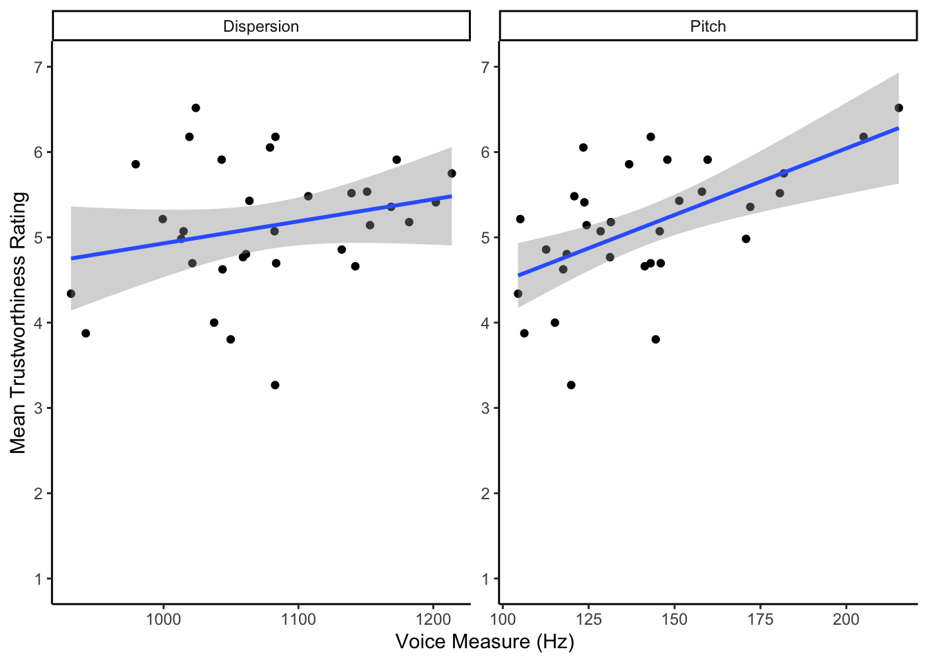

Scatterplot showing the relationship between the voice measures of Dispersion (left) and Pitch (right) and Mean Trustworthiness Rating

Figure 14.1: Scatterplot showing the relationship between the voice measures of Dispersion (left) and Pitch (right) and Mean Trustworthiness Rating

Answer me:

According to the scatterplot, there appears to be a between both pitch and trustworthiness and dispersion and trustworthiness though the relationship with seems stronger.

The scatterplot

ggplot() + geom_point()
geom_smooth(method = "lm")
coord_cartesian or scale_y_continuous
facet_wrap(scales = "free")
did you know also that you can control the number of columns and rows in a facet_wrap by adding nrow and ncol?
for example, facet_wrap(~variable, nrow = 1, ncol = 2)

The interpretation

The first consideration is direction. Remember that a positive relationship means as scores on one variable increase so do scores on the other variable, and negative means as scores on one variables increase, scores on the other variable decrease.
The second consideration is strength: strong, medium or weak.

14.3.6 Task 6: Spreading the data with `pivot_wider()`

Ok so we are starting to get an understanding of our data and we want to start thinking about the regression. However, the regression would be easier to work with if Pitch and Dispersion were in separate columns. So I know we just joined the columns together to create the figure and now we are splitting them to do the analyse and that might seem odd. There are ways around this that you will develop in future years but when learning it can help just to keep everything systematic and really highly processed. So sometimes you will see funny moves like this. But remember, if the code works and does what you need, then the only bad code is no code

Using the pivot_wider() function, create a new tibble where Pitch and Dispersion data have been split into two columns called Pitch and Dispersion respectively.
We used pivot_wider() to spread data in Chapter 5 when creating the difference of two groups so maybe refer back then to see how to input the columns, but there is also information in the hint below.

pivot_wider() needs the data, name of the categorical column to spread, and the name of the data to spread
pivot_wider(data, names_from = "column_name", values_from = "column_name")

14.3.7 Task 7: The Regressions

Ok we are almost at the point when we need to do the regression. We should always think about assumptions but as that is covered in the lecture series we will mostly leave that there for now. That said, one assumption we can roughly and quickly look at is the correlation between Pitch and Dispersion, remembering the issue of multicollinearity - if predictors are highly correlated (r > .8 for example then it is impossible to tease apart their unique contributions). So, now, run a code using cor.test() to calculate the correlation between Pitch and Dispersion and then fill in this statement.

The correlation between Pitch and Dispersion is which would suggest that we have no issues with multicollinearity as our two predictors are only slightly correlated. So nothing to worry about there.

Right, now let's do some regression analysis. We will first do two simple linear regressions (one for each predictor), and then we will do a multiple linear regression using both predictors.

The lm() function in R is the main function we will use to estimate a Linear Model (hence the function name lm). The function takes the format of:

lm(dv ~ iv, data = my_data) for simple linear regression
lm(dv ~ iv1 + iv2, data = my_data) for multiple linear regression

Now, use the lm() function to run the following three regression models.

Simple Linear Regression

Run the simple linear regression of predicting trustworthiness mean ratings from Pitch and store the model in mod_pitch
Run the simple linear regression of predicting trustworthiness mean ratings from Dispersion and store the model in mod_disp

Multitple Linear Regression

Run the multiple linear regression of predicting trustworthiness mean ratings from Pitch and Dispersion, and store the model in mod_pitchdisp

Correlations

You could argue that you should use a Spearman correlation for the correlation between Pitch and Dispersion because the scales are very different although measured both in (Hz), though it would not be wrong to use Pearson here either as it is still the same scale.
You may need to refer back to Chapter 10 on correlations to remember how to use cor.test().

Regressions

The functions would be something like:

lm(trust_column ~ pitch_column, data = my_data) for simple linear regression
lm(trust_column ~ pitch_column + dispersion_column, data = my_data) for multiple linear regression

14.3.8 Task 8: Model interpretations

Now let's look at the results of each model in turn, using the function summary(), e.g. summary(mod_pitch), and try to interpret them based on what you already know about regression outputs from the lectures.

Let's start by looking at the mod_pitch model together.

summary(mod_pitch)

## 
## Call:
## lm(formula = mean_rating ~ Pitch, data = joined_wide)
## 
## Residuals:
##      Min       1Q   Median       3Q      Max 
## -1.52562 -0.30181  0.04361  0.33398  1.20492 
## 
## Coefficients:
##             Estimate Std. Error t value Pr(>|t|)    
## (Intercept) 2.921932   0.583801   5.005  2.3e-05 ***
## Pitch       0.015607   0.004052   3.852 0.000573 ***
## ---
## Signif. codes:  0 '***' 0.001 '**' 0.01 '*' 0.05 '.' 0.1 ' ' 1
## 
## Residual standard error: 0.6279 on 30 degrees of freedom
## Multiple R-squared:  0.3309, Adjusted R-squared:  0.3086 
## F-statistic: 14.83 on 1 and 30 DF,  p-value: 0.0005732

From the output we can see that this model, when relating to the population, would predict approximately 30.86% of the variance in trustworthiness ratings (Adjusted-R^2 = 0.3086). We could also say that a linear regression model revealed that pitch significantly predicted perceived trustworthiness scores in male voices in that as pitch increased so does perceived trustworthiness (\(b\) = 0.0156, t(30) = 3.852, p < .001). (Remember that these are unstandardised coefficients so the "Estimate" would mean that a one unit change in pitch would result in a 0.0156 unit change in perceived trust, a rather small change.)

Overall, looking at this model with just Pitch as a predictor, we have a regression model of small to medium prediction (i.e. explained variance) but it is significantly better than a model using the mean value of trust ratings as a prediction - as shown by the F-test being significant. Remember from the lectures that the default model is where every predicted value of Y is the mean of Y; we called this the mean model. So our new model is better than using that model based on the mean.

Worth also pointing out here that in a simple linear regression the F-test and the t-value for the predictor are the same based on t^2 = F, as seen earlier in this book. For example, looking at the values above, we see that 3.852 \(\times\) 3.852 = 14.83. Just again goes to show that there is a link between the tests we have been looking at.

Ok, based on that knowledge, answer the following questions about the two remaining models.

The model of just dispersion as a predictor would explain approximately
In fact, the model of just dispersion is and therefor as a model
Looking at the multiple linear regression model, the explained variance is and as such explains variance than the pitch only model.

We have added a brief interpretation of the models in the solution to this task as well so it might be worth reading that to make sure you are understanding the outputs.

What the above should remind you is that it is not the case that simply putting all the possible predictors into a model will make it a better model. For every predictor you add there is a penalty associated with the Adjusted-R^2 and if the explained variance attributable to the new predictor is not greater than the penalty to overall explained variance then you may actually end up with a worse model despite having more predictors. We touched briefly in the lecture on using the anova(model1, model2) approach to compare models; something like this:

anova(mod_pitch, mod_pitchdisp)

Which gives the following output:

Res.Df	RSS	Df	Sum of Sq	F	Pr(>F)
30	11.82665	NA	NA	NA	NA
29	11.48600	1	0.3406532	0.8600855	0.3613695

And shows no significant difference between these two models. We will look at model comparison more in the coming months and years but it is always good to keep the rule of parsimony in mind! The simpler the better.

14.3.9 Task 9: Making predictions

Congratulations! You have successfully constructed a linear model relating trustworthiness to pitch and dispersion and you can think about applying this knowledge to other challenges - perhaps go look at female voices? However, one last thing you might want to do that we will quickly show you is how to make a prediction using the predict() function. One way you use this, though see the solution to the chapter for alternatives, is:

predict(model, newdata)

where newdata is a tibble with new observations/values of X (e.g. pitch and/or dispersion) for which you want to predict the corresponding Y values (mean_rating). So let's try that out now.

Make a tibble with two columns, one called Pitch and one called Dispersion - exactly as spelt in the model. Give Pitch a value of 150 Hz (quite a high voice) and give Dispersion a value of 1100 Hz - somewhere in the middle. We saw how to create tibbles in Chapter 5 using the tibble() function so you might need to refer back to that.
Now put that tibble, newdata, into the predict() function and run it on the mod_pitchdisp. Follow the above format of model as first argument and tibble of new values as second argument.

Now, based on the output try to answer this question:

To one decimal place, what is the predicted trustworthiness rating of a person with 150 Hz Pitch and 1100 Hz Dispersion -

tibble(Pitch = Value, Dispersion = Value)
predict(mod_pitchdisp, newdata)
Note: Alternative ways to enter the data are in the solution for this task.

WAIT! - Didn't we just say that the mod_pitchdisp model is not as good as mod_pitch. Yep. We did and that is actually what the model comparison shows above as well, but we wanted to show you how to enter different predictors into the predict() function. So whilst this is a good teaching aid, you are 100% correct in thinking that in reality we would be better making predictions with just the mod_pitch model as it explains more variance overall. Well done for spotting that!

Job Done - Activity Complete!

Great! Now you know how to make predictions why not try a few more. Choose some pitch values see what you get! Go record your voice. Extract the pitch using something like PRAAT. Put it in the predict() function. Get a rating of trustworthiness for your voice. Go run a study that has your voice rated for trustworthiness and see how close the model was. Given the explained variance is not great it probably won't be that close but you start to see how, in principle, the idea of regression and prediction of relationships works. The greater the explained variance of your predictors, the better your prediction will be for a novel participant/observation/event!

One last thing:

Before ending this section, if you have any questions, please post them on the available forums or speak to a member of the team. Finally, don't forget to add any useful information to your Portfolio before you leave it too long and forget. Remember the more you work with knowledge and skills the easier they become.

14.4 Assignment

This is a summative assignment and as such, as well as testing your knowledge, skills, and learning, this assignment contributes to your overall grade for this semester. You will be instructed by the Course Lead on Moodle as to when you will receive this assignment, as well as given full instructions as to how to access and submit the assignment. Please check the information and schedule on the Level 2 Moodle page.

14.5 Solutions to Questions

Below you will find the solutions to the questions for the Activities in this chapter. Only look at them after giving the questions a good try and speaking to the tutor about any issues.

14.5.1 InClass Activities

14.5.2 Task 1

library("broom")
library("tidyverse")

ratings <- read_csv("voice_ratings.csv")
acoustics <- read_csv("voice_acoustics.csv")

Return to Task

14.5.3 Task 2

We are calling the new tibble ratings_tidy. We did not state what to call it as by now you can make that decision yourself. Just remember that when debugging your analysis paths from now on, the tibble names might not match up so, you may need to do a little bit of backtracking to see where tibbles were created.

ratings_tidy <- pivot_longer(ratings, 
                              names_to = "participant", 
                              values_to = "rating", 
                              cols = "P1":"P28")

Return to Task

14.5.4 Task 3

ratings_mean <- ratings_tidy %>% 
  group_by(VoiceID) %>% 
  summarise(mean_rating = mean(rating))

Return to Task

14.5.5 Task 4

joined <- inner_join(ratings_mean, 
                     acoustics, 
                     "VoiceID") %>% 
  filter(sex == "M")

Return to Task

14.5.6 Task 5

The following code:

ggplot(joined, aes(value, mean_rating)) +
  geom_point() +
  geom_smooth(method = "lm") +
  scale_y_continuous(breaks = c(1:7), limits = c(1,7)) +
  facet_wrap(~measures, nrow = 1, ncol = 2, scales = "free") +
  theme_classic()

Will gives the below figure:

## `geom_smooth()` using formula 'y ~ x'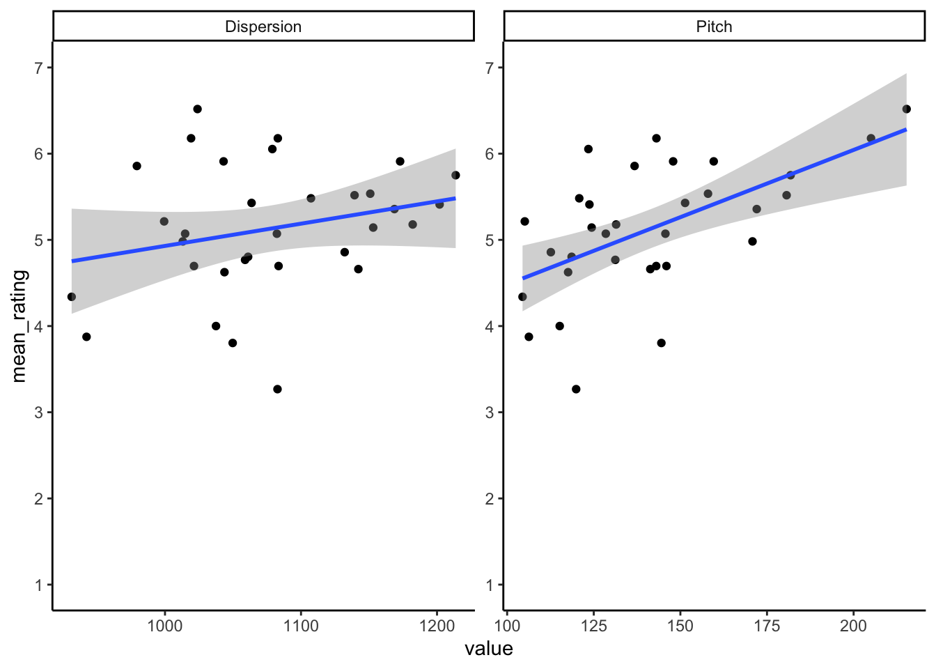

Figure 14.2: Scatterplot showing the relationship between the voice measures of Dispersion (left) and Pitch (right) and Mean Trustworthiness Rating

Return to Task

14.5.7 Task 6

pivot_wider() is the reverse of pivot_longer()
It takes in the data and you tell it which values you want to spread and by which column
Order is normally, data, names_from, values_from.

joined_wide <- joined %>% pivot_wider(names_from = "measures",
                                      values_from = "value")

Return to Task

14.5.8 Task 7

Simple Linear Regression - Pitch

The pitch model would be written as such:

mod_pitch <- lm(mean_rating ~ Pitch, joined_wide)

And gives the following output:

summary(mod_pitch)

## 
## Call:
## lm(formula = mean_rating ~ Pitch, data = joined_wide)
## 
## Residuals:
##      Min       1Q   Median       3Q      Max 
## -1.52562 -0.30181  0.04361  0.33398  1.20492 
## 
## Coefficients:
##             Estimate Std. Error t value Pr(>|t|)    
## (Intercept) 2.921932   0.583801   5.005  2.3e-05 ***
## Pitch       0.015607   0.004052   3.852 0.000573 ***
## ---
## Signif. codes:  0 '***' 0.001 '**' 0.01 '*' 0.05 '.' 0.1 ' ' 1
## 
## Residual standard error: 0.6279 on 30 degrees of freedom
## Multiple R-squared:  0.3309, Adjusted R-squared:  0.3086 
## F-statistic: 14.83 on 1 and 30 DF,  p-value: 0.0005732

Simple Linear Regression - Dispersion

The Dispersion model would be written as such:

mod_disp <- lm(mean_rating ~ Dispersion, joined_wide)

And gives the following output:

summary(mod_disp)

## 
## Call:
## lm(formula = mean_rating ~ Dispersion, data = joined_wide)
## 
## Residuals:
##      Min       1Q   Median       3Q      Max 
## -1.87532 -0.41300 -0.02435  0.29850  1.52664 
## 
## Coefficients:
##             Estimate Std. Error t value Pr(>|t|)
## (Intercept) 2.345300   1.982971   1.183    0.246
## Dispersion  0.002584   0.001836   1.407    0.170
## 
## Residual standard error: 0.7434 on 30 degrees of freedom
## Multiple R-squared:  0.06191,    Adjusted R-squared:  0.03064 
## F-statistic:  1.98 on 1 and 30 DF,  p-value: 0.1697

Multiple Linear Regression - Pitch + Dispersion

The model with both Pitch and Dispersion as predictors would be written as such:

mod_pitchdisp <- lm(mean_rating ~ Pitch + Dispersion, joined_wide)

And gives the following output:

summary(mod_pitchdisp)

## 
## Call:
## lm(formula = mean_rating ~ Pitch + Dispersion, data = joined_wide)
## 
## Residuals:
##      Min       1Q   Median       3Q      Max 
## -1.54962 -0.36428  0.04033  0.36327  1.18915 
## 
## Coefficients:
##             Estimate Std. Error t value Pr(>|t|)   
## (Intercept) 1.444290   1.697362   0.851  0.40179   
## Pitch       0.014855   0.004142   3.586  0.00121 **
## Dispersion  0.001470   0.001585   0.927  0.36137   
## ---
## Signif. codes:  0 '***' 0.001 '**' 0.01 '*' 0.05 '.' 0.1 ' ' 1
## 
## Residual standard error: 0.6293 on 29 degrees of freedom
## Multiple R-squared:  0.3501, Adjusted R-squared:  0.3053 
## F-statistic: 7.813 on 2 and 29 DF,  p-value: 0.001931

Return to Task

14.5.9 Task 8

A brief explanation:

From the models you can see that the Dispersion only model is not actually significant (F(1,30) = 1.98, p = .17) meaning that it is not actually any better than using the model that just predicts the mean values. This is backed up by it only explaining around 3% of the variance. Looking at the multiple linear regression model which contains both pitch and dispersion we can see that it is a significant model ((F(2,29) = 7.81, p = .002) explaining 30.5% of the variance). However looking at the p-values of the coefficients, in the column labelled Pr(>|t|), only pitch is a significant predictor in this model (noting that the p-value for pitch (p = .001) is less than \(\alpha\) = .05, but the p-value for dispersion is not, (p = .361)). In addition, we see that actually the multiple regression model has smaller predictive ability than the pitch alone model. As such, there is an arguement to be made that the pitch alone model is the best model in the current analysis but in future you might want to actually compare the models using the anova(model1, model2) approach.

Return to Task

14.5.10 Task 9

Solution Version 1

newdata <- tibble(Pitch = 150, Dispersion = 1100)

predict(mod_pitchdisp, newdata)

##        1 
## 5.289819

Solution Version 2

predict(mod_pitchdisp, tibble(Pitch = 150, 
                              Dispersion = 1100))

##        1 
## 5.289819

Solution Version 3

And if you want to bring it out as a single value, say for a write-up, you could do the following
This approach may give out a warning about a deprecated function meaning that this won't work in future updates but for now it is ok to use.

predict(mod_pitchdisp, tibble(Pitch = 150, 
                              Dispersion = 1100)) %>% 
  tidy() %>% 
  pull() %>% 
  round(1)

## Warning: 'tidy.numeric' is deprecated.
## See help("Deprecated")

## Warning: `data_frame()` was deprecated in tibble 1.1.0.
## Please use `tibble()` instead.
## This warning is displayed once every 8 hours.
## Call `lifecycle::last_warnings()` to see where this warning was generated.

## [1] 5.3

or even just:

predict(mod_pitchdisp, tibble(Pitch = 150, 
                              Dispersion = 1100)) %>% 
  pluck("1") %>% 
  round(1)

## [1] 5.3

Return to Task

Chapter Complete!

Lab 14 Regression

14.1 Overview

14.2 PreClass Activity

14.2.1 Read

14.3 InClass Activity

14.3.1 Task 1: Setup

14.3.2 Task 2: Restructuring the ratings

14.3.3 Task 3: Calculate mean trustworthiness rating for each voice

14.3.4 Task 4: Joining the Data together

14.3.5 Task 5: Scatterplot

14.3.6 Task 6: Spreading the data with pivot_wider()

14.3.7 Task 7: The Regressions

14.3.8 Task 8: Model interpretations

14.3.9 Task 9: Making predictions

14.4 Assignment

14.5 Solutions to Questions

14.5.1 InClass Activities

14.5.2 Task 1

14.5.3 Task 2

14.5.4 Task 3

14.5.5 Task 4

14.5.6 Task 5

14.5.7 Task 6

14.5.8 Task 7

14.5.9 Task 8

14.5.10 Task 9

14.3.6 Task 6: Spreading the data with `pivot_wider()`